Introductory concepts

This section covers a series of introductory concepts that are important for the course and for observational astronomy in general. It is not intended to be thoroughly exhaustive, but rather to provide a basic understanding of the topics that will be covered in more detail later in the course. Further reading is provided at the end of the section and as links throughout the text.

Coordinate systems

Anybody who has spent some time looking at the sky in a dark place at night has noticed that the stars, planets, and other astronomical objects seem to be arranged on the “surface” of a sphere that rotates around a point. If we take a long-exposure photograph centred around that “celestial pole” we will see that the stars move in arcs.

Of course, we understand why this is happening: the sky rotates as a result of the rotation of the Earth, with the Earth’s axis of rotation —when projected on the sky— defining the point around which the celestial sphere rotates. And the stars are not all really on the same plane, but rather at different distances from us. But those distances are so vast that perspective renders them all on a what appears to be a single surface.

That said, it is convenient for many purposes to think of the sky as a sphere that rotates around a given axis, and the celestial objects being placed on the surface of that sphere.

Definitions

Let’s start with some basic definitions. Imagine a spherical surface with unit radius. We draw a line that passes through the centre of the sphere, \(C\) and intersects the surface at two points, \(P\) and \(P'\) which we will call the poles. Next we define a plane that passes through the centre of the sphere and is perpendicular to the line that connects the two poles. This plane intersects the surface of the sphere at a circle which we will call the fundamental circle.

Now let’s define a point \(A\) on the surface of the sphere. We can draw a circle that passes through both poles and \(A\) (note that this circle is centred on \(C\)). This circle intersects the fundamental circle at a point \(B\).

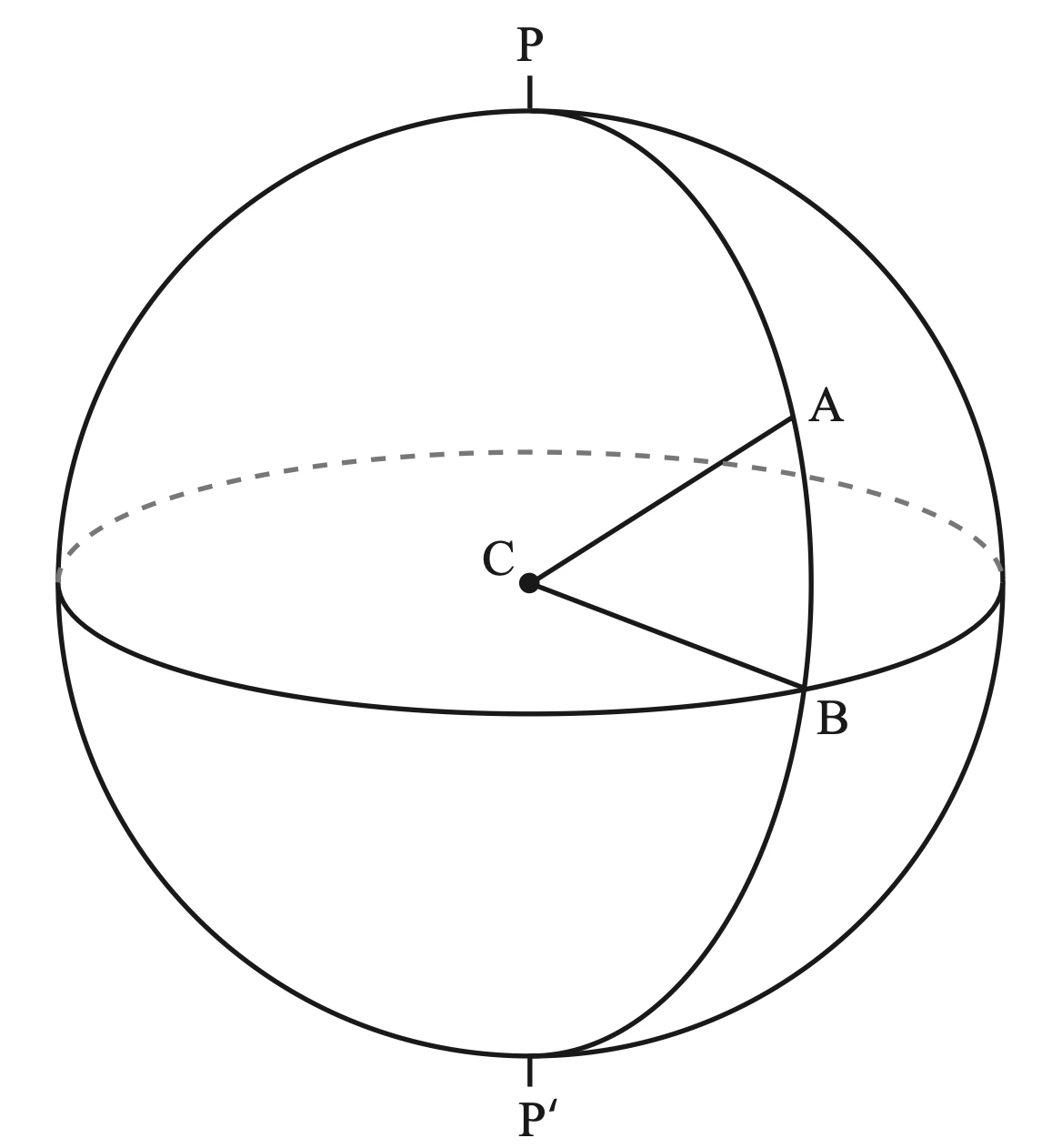
Source: Observational Astronomy, Birney et al. (2nd ed.)

Let’s now draw a circle that is parallel to the fundamental circle and intersects the surface of the sphere at \(A\). Finally, let’s define another point \(D\) on the fundamental circle.

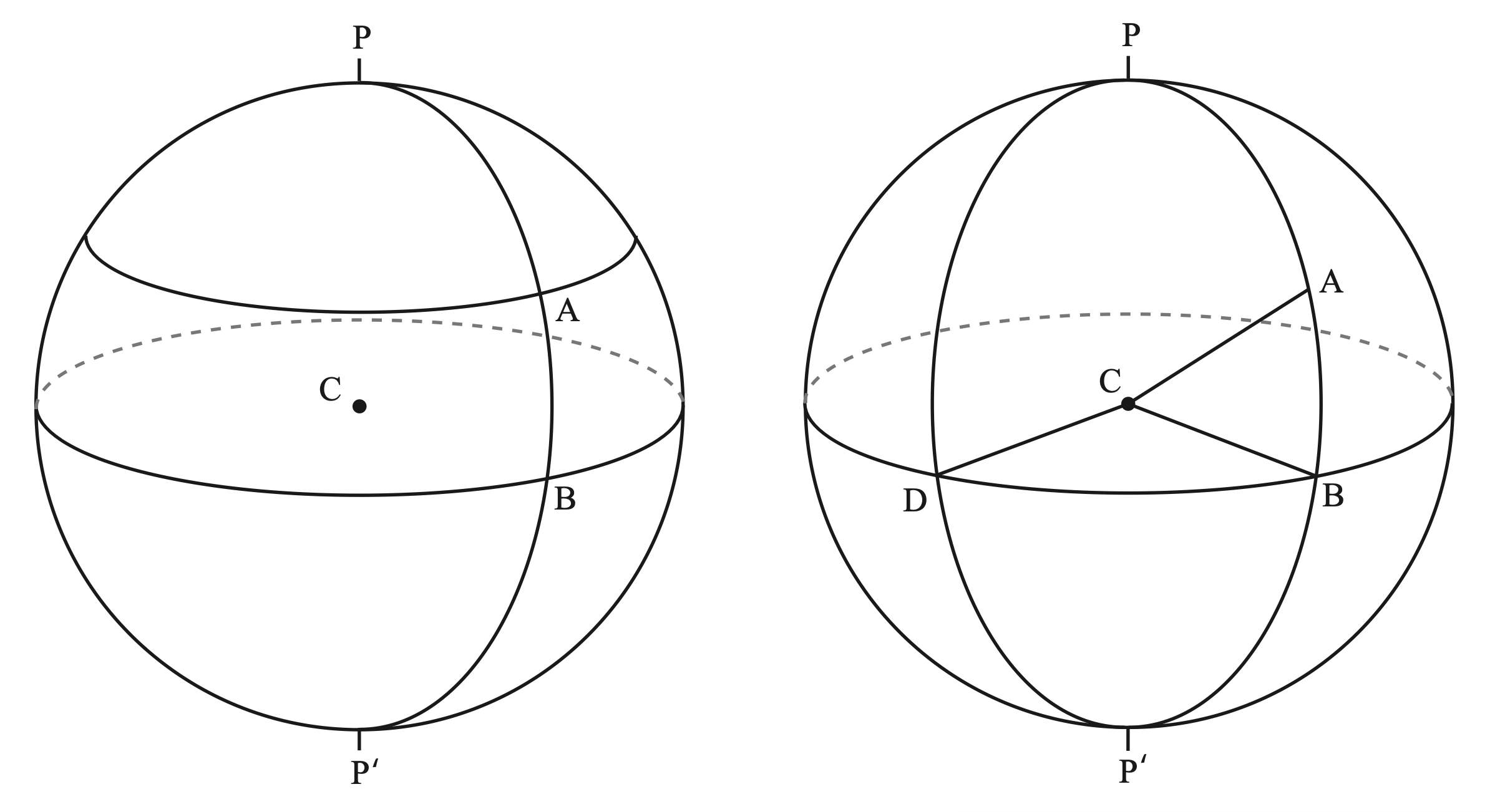
Source: Observational Astronomy, Birney et al. (2nd ed.)

The point \(A\) can now be defined using two angles: the angle \(\angle ACB\) and the angle \(\angle DCB\). We can also define and important concepts: a great circle is one defined by a plane that passes through the centre of the sphere. All great circles have equal length and are the largest possible circle than can be drawn on the sphere. A small circle is a circle defined on the sphere that is not a great circle. In our example above the circles \(PABP'\) and \(PDP'\) are great circles, as well as the fundamental circle. The circle that is parallel to the fundamental circle and passes through \(A\) is a small circle. The shortest distance between two points on the surface of a sphere is always along a great circle, a concept that is sometimes counter-intuitive. The length of a small circle that is parallel to the fundamental circle decreases with the cosine of the angle (e.g., \(\cos(ACB)\)).

Spherical trigonometry

Spherical trigonometry is the branch of mathematics that studies with the relationships between angles and distances on the surface of a sphere. While many concepts may seem similar to planar (or Euclidean) trigonometry, there are important differences. Let’s start by defining a triangle from the intersection of three great circles:

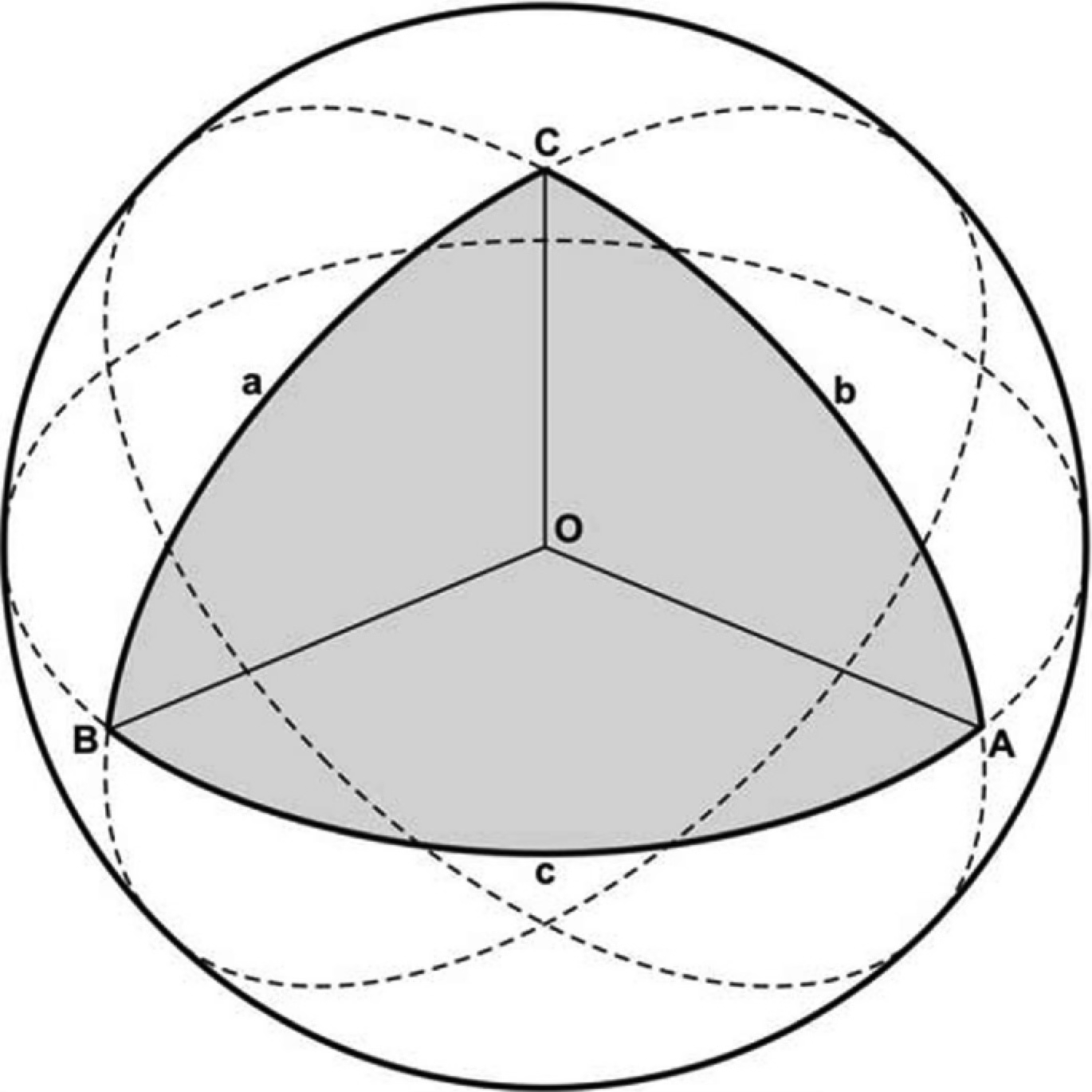
Source: Observational Astronomy, Birney et al. (2nd ed.)

Angles on a spherical triangle are denoted with capital latin letters. In our case \(A\), \(B\), and \(C\) are the angles at the vertices of the triangle. \(A\) (and \(B\) and \(C\)) is the angle between the two planes that intersect the sphere at vertex \(A\). Angles are measured in radians

The sides of the triangle are also measured in radians and measured by the angle that it subtends at the centre. The sides are denoted with lower case letters, so \(a\) is the side opposite to angle \(A\), \(b\) is the side opposite to angle \(B\), and \(c\) is the side opposite to angle \(C\).

By definition a spherical triangle angle is less than \(\pi\) radians so

\[ \pi < A+ B+ C < 3\pi \]

while the sides are less than \(\pi\) radians, so

\[ 0 < a+ b+ c < 2\pi \]

The most important rule of spherical trigonometry is the law of cosines. A proof of this law (and other relationships that we will see below) can be found in many textbooks on spherical astronomy, for example in Chapter 1 of Smart’s Textbook on Spherical Astronomy. The law of cosines applies to each angle so we can write three expressions such as:

\[\begin{split} \begin{eqnarray*} \cos a &=& \cos b \cos c + \sin b \sin c \cos A \\ \cos b &=& \cos a \cos c + \sin a \sin c \cos B \\ \cos c &=& \cos a \cos b + \sin a \sin b \cos C \end{eqnarray*} \end{split}\]

From the law of cosines we can derive the law of sines:

\[ \frac{\sin A}{\sin a} = \frac{\sin B}{\sin b} = \frac{\sin C}{\sin c} \]

These two expressions are the base of spherical trigonometry can be used to derive any additional relationships. For right spherical triangles (triangles in which one angle is formed by the intersection of two perpendicular planes) we can also make use of Napier’s rules which we won’t cover here but that are essential for solving problems in astronomical spherical trigonometry, where many triangles are right triangles.

Important

Spherical trigonometry applies only to spherical triangles, that is, triangles defined by the intersection of three great circles. Triangles formed by the intersection of small circles do not follow these rules.

Separations on the sphere

A typical problem in spherical trigonometry consists on measuring the distance (separation) between two points on the surface of a sphere. In particular, consider the distance \(\beta\) in the following case:

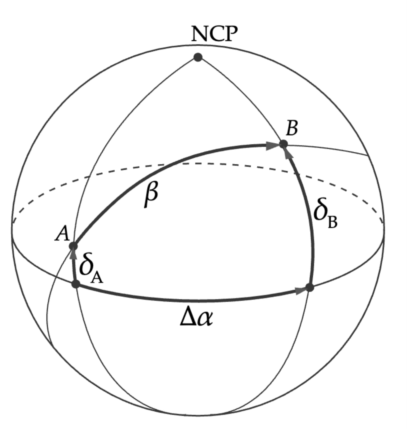
Source: Observational Astronomy, Birney et al. (2nd ed.)

As we will see, \(A\) and \(B\) are defined using reference points that are natural in spherical coordinate systems. While the sides labelled with \(\alpha\) and \(\beta\) make reference to an equatorial coordinate system, this is a general case and the solution is generally valid. We’ll leave the proof of this experiment to the reader (hint: consider the triangle defined by the \({\rm NCP}-B\) and \(AB\) great circles and the fundamental plane, and use the Napier’s rules).

\[\begin{split} \begin{eqnarray*} \beta^2 &=& \Delta\delta^2 + \cos^2 \bar\delta \Delta\alpha^2 \\ \bar\delta &=& \dfrac{\delta_A + \delta_B}{2} \\ \end{eqnarray*} \end{split}\]

Horizontal coordinates

The simplest type of coordinates is called horizontal (also altitude-azimuth or alt-az). Imagine that you are standing on the surface of the Earth in a place where you can all the way to the horizon. The point just above your head is called the zenith. The one just below your feet is called the nadir. These two points defined the poles of the horizontal coordinate system while the horizon is the fundamental circle. If we have a point \(S\) on the sky, we can define its position with two coordinates: altitude (\(h\)) and azimuth (\(A\)). Altitude is the simplest one and is just the angle, perpendicular to the horizon, between the horizon and the point. For the azimuth we need to define an arbitrary reference point on the horizon. We chose the North cardinal point (the direction of the North pole) and measure the angle from there, going clockwise (azimuth angles increase from North towards East).

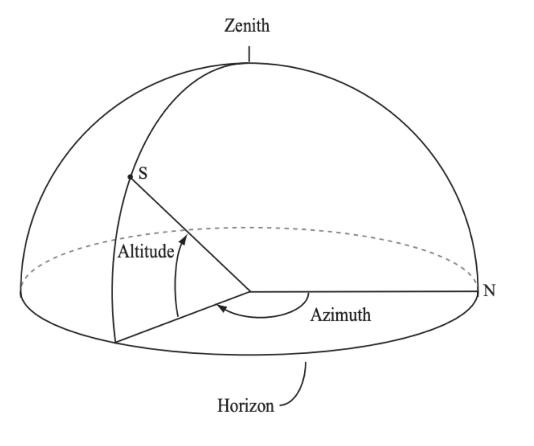
Source: Observational Astronomy, Birney et al. (2nd ed.)

Warning

There is no strong convention on how to define the azimuth angle. Some people define it as the angle from the South cardinal point, going clockwise. When dealing with alt-az coordinates always make sure that you know how the azimuth angle is defined. Similarly, the letters \(h\) and \(A\) are not universally used to denote altitude and azimuth, respectively.

A critical thing to realise is that the horizontal coordinates of an object change during the night as the sky rotates. Because of that we need an additional datum, the time of observation, to fully define the position of such object. The coordinates of the object will also depend on the location of the observer on the Earth. Imagine an observer on the equator observing a star that is at the zenith. That observer will measure an altitude of 90 degrees. Now imagine an observer at the North (or South) pole observing the same star at the same time: they will measure an altitude of 0 degrees!

Before we move on, we can introduce a few additional concepts based on the horizontal coordinate system. The zenith distance (\(z\)) is the distance between the point we are trying to measure and the zenith. Twilights are defined as the moment in which the Sun reaches a certain point below the horizon. The most common definitions are civil twilight (when the Sun is 6 degrees below the horizon), nautical twilight (12 degrees below the horizon), and astronomical twilight (18 degrees below the horizon).

Equatorial coordinates

While horizontal coordinates are easy to understand but are not practical to define the position of celestial object in a way that is independent of the observer’s location and time. For that we need to define a coordinate system that is fixed with respect to the stars. The most common system that meets this requirement is the equatorial coordinate system.

As we did before, let’s imagine a celestial sphere, centred on the Earth, but in this case the poles will be the North and South celestial poles (NCP, SCP), that is, the points on the celestial sphere that are aligned with the Earth’s axis of rotation. The fundamental circle in this system is called the celestial equator. For a given point \(S\) on the sphere we define its position with two angles: declination (Dec or \(\delta\)) and right ascension (RA or \(\alpha\)). The declination is measured from the celestial equator following the great circle that passes through \(S\) and the poles (declination is positive towards the NCP). As with horizontal coordinates we now need to define a reference point for the right ascension. We chose the point on the celestial equator on which the Sun is at the vernal (Spring) equinox, which we call the vernal point. RA increases along the celestial equator clockwise when looking from the NCP. The units of RA are usually hours, minutes, and seconds (1 hour = 15 degrees) and declination is always measured in degrees.

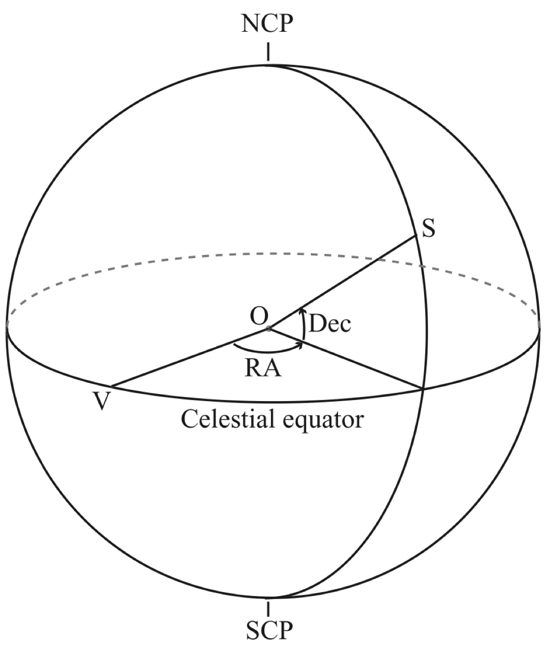
Source: Observational Astronomy, Birney et al. (2nd ed.)

Since the sky rotates around the polar axis, the declination of an object never changes, and as the vernal point also rotates, the right ascension of the object is also constant. The equatorial coordinates of an object are fixed regardless of the observer’s location or time of observation (as we’ll see, things are a bit more complicated, but for now we can assume that this is true).

Note

Technically the equatorial system that we have defined is called Geocentric Celestial Reference System since the centre of the coordinate system is assumed to be the centre of mass of the Earth. As we’ll see later, other equatorial systems can be defined with centres at other points, such as the barycentre of the Solar System.

We can put the horizontal and equatorial coordinate systems together in a single diagram to see how they relate to each other. Here the celestial equator and horizon form an angle equal to the latitude of the observer’s location on the Earth. The angle \(ZS\) is the zenith distance and the angle \(PS\) along the great circle perpendicular to the celestial equator is the hour angle. The circle that passes through the zenith and the poles is called the local meridian.

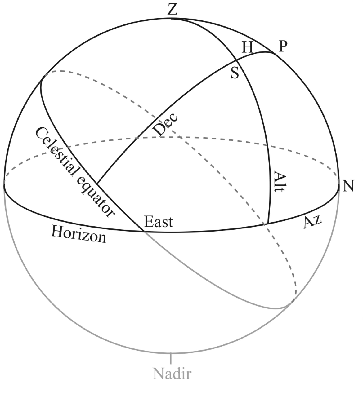
Source: Observational Astronomy, Birney et al. (2nd ed.)

Hour angle

We will more properly introduce sidereal time later, but for now let’s just define local sidereal time (LST) as the angle between the local meridian and the vernal point. LST is measured in hours and is zero when the vernal point crosses the local meridian.

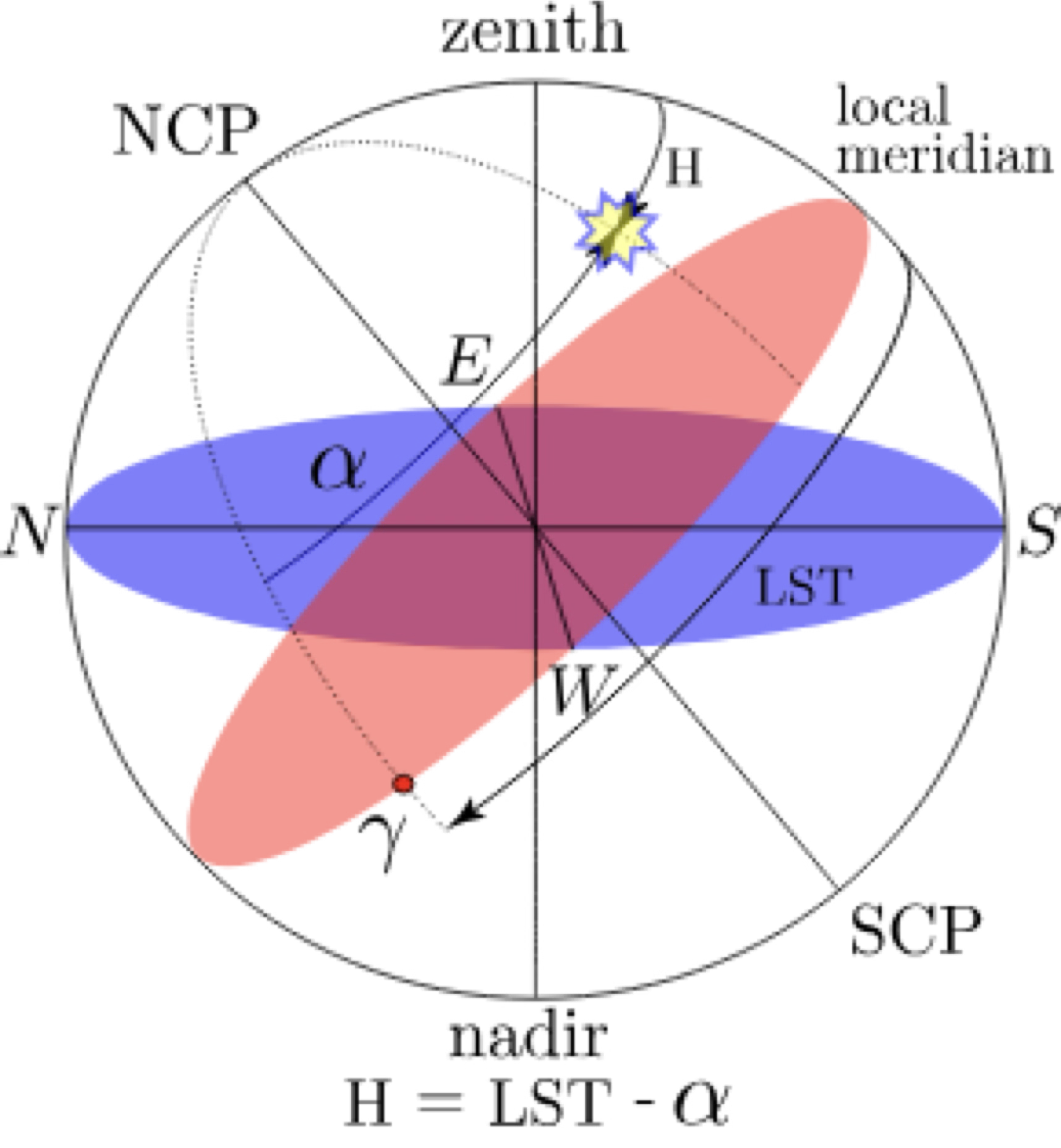
We then define the hour angle (\(H\)) as the angle between the local meridian and the object. From the diagram above it’s clear that the H and the LST are related by \(H={\rm LST}-\alpha\). The hour angle is measured in hours and increases towards the West. Since an object on the sky will move from East to West, a negative hour angle indicates that the object is rising and a positive hour angle indicates that the object is setting. The hour angle is zero when the object crosses the local meridian, at which point the local sidereal time is the same as the right ascension of the object.

Other coordinate systems

The horizontal and equatorial coordinate systems are the most commonly used in astronomy, but there are many other coordinate systems that can be defined. Here we quickly introduce a few of them.

Ecliptic coordinates

Ecliptic coordinates are defined using the plane of the ecliptic (the average plane of the Earth’s orbit around the Sun) as the fundamental circle. The ecliptic longitude \(\lambda\) is measured along the ecliptic from the vernal point, and the ecliptic latitude \(\beta\) is measured perpendicular to the ecliptic plane. The ecliptic coordinates are useful for defining the position of objects in the Solar System, such as planets and comets.

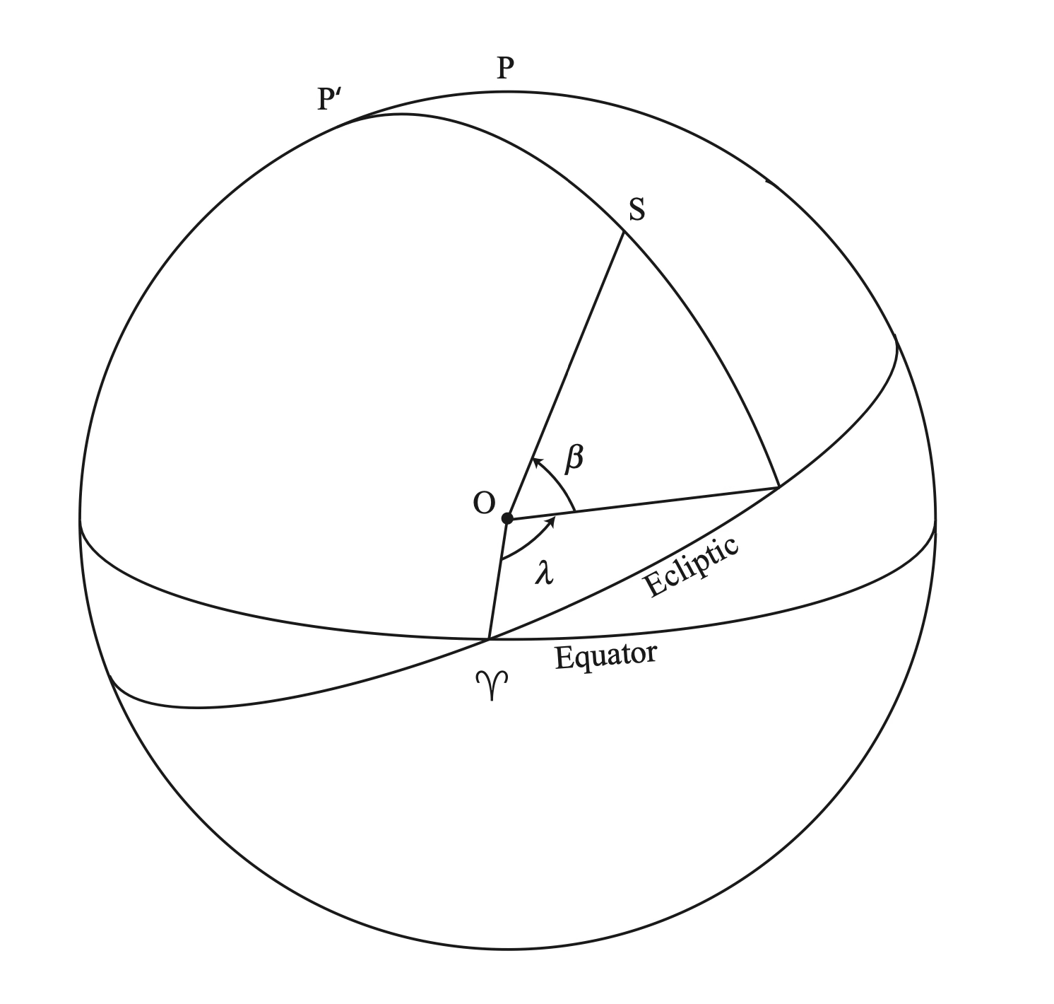
Source: Observational Astronomy, Birney et al. (2nd ed.)

Galactic coordinates

Galactic coordinates provide a more natural way to specify the position of objects in the Milky Way. The fundamental circle is defined from the plane of the Milky Way (this is not trivial and a convention is used) with the Galactic Poles as the axis of the system. The Galactic latitude \(b\) is measured perpendicular to this plane and indicates the angle of the object with respect to the disk of the Milky Way (and so, most stars have relatively small Galactic latitudes). The Galactic longitude \(l\) is measured with respect to the direction of the Galactic centre.

Source: Observational Astronomy, Birney et al. (2nd ed.)

Precession of the equinoxes

The gravitational pull of the Sun and the Moon on the Earth causes it axis of rotation to wobble over time. The polar axis describes a circle on the celestial sphere with a period of about 26,000 years. This phenomenon is called precession of the equinoxes. The effect of the precession in the equatorial coordinate system is that as polar axis changes so does the celestial equator and the location of the vernal point (which is defined as one of the point in which the ecliptic intersects the celestial equator). Although the change due to precession may seem small, it is in the order of \(\sim 50\) arcseconds per year, which is significant for many astronomical applications. This means that the equatorial coordinates of an object will change over time as the vernal point changes. To account for this effect, astronomers refer to the equatorial coordinates of an object at a given epoch. Most coordinates these days are referred to the position of the vernal point in the Julian date 2000 (usually referred as J2000) but older catalogues may use B1950 (Besselian epoch 1950.0).

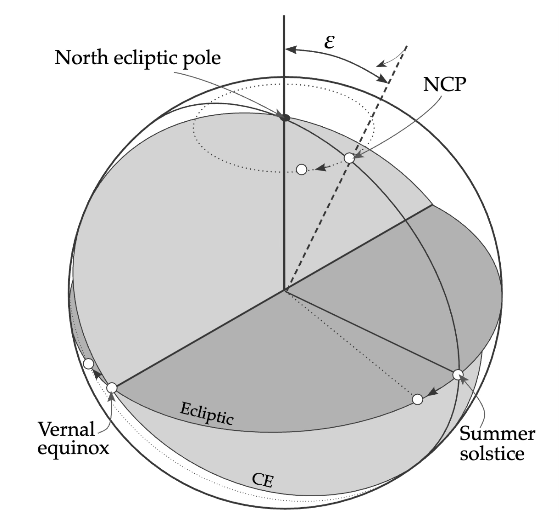
Source: Observational Astronomy, Birney et al. (2nd ed.)

Additional effects such as nutation also affect the alignment of the celestial pole, but usually these effects are small enough that they can be ignored for most applications.

The inconvenience of the shifting of the vernal equinox has lead to the establishment of the International Celestial Reference System (ICRS) and other systems that are defined with respect to very stable reference points (usually distant radio sources). The ICRS is centred on the barycentre of the Solar System while the Geocentric Celestial Reference System (GCRS) is centred on the centre of mass of the Earth and is useful for calculating the position of near-Earth objects.

The ICRS is defined so that its orientation matches the direction of the vernal point in J2000 within approximately 23 milliarcseconds. Because of that, for most applications one can ignore differences between J200 and ICRS. These differences are important, however, when carrying out transformations to other coordinate systems.

Coordinate transformations

We often need to transform from one coordinate system to another. Coordinate transformations can be derived using the basic rules of spherical trigonometry, and transformations between many common coordinate systems can be found in textbooks and online. By far the most common coordinate transformation is between equatorial and horizontal coordinates, which is especially useful when planning observations to determine the altitude of an object at the site of observation during the night. If we refer to the figure relating equatorial and horizontal coordinates, we can write the following equations:

\[\begin{split} \begin{eqnarray*} \sin h &=& \sin \delta \sin \phi + \cos \delta \cos \phi \cos {\rm HA} \\ \tan A &=& \dfrac{\sin {\rm HA}}{\cos {\rm HA} \sin \phi - \tan \delta \cos \phi} \\ \end{eqnarray*} \end{split}\]

where \({\rm HA} = {\rm LST}-\alpha\), \(h\) is the altitude, \(A\) is the azimuth, \(\delta\) is the declination, and \(\phi\) is the latitude of the observer. There is an implicit ambiguity in the azimuth angle, which can be resolved by using the two-argument arctangent function, \({\rm atan2}(y,x)\). In this form \(A=-{\rm atan2}(y, x)\) with

\[\begin{split} \begin{eqnarray*} y &=& \sin {\rm HA}\cos\delta \\ x &=& -\sin\phi \cos\delta \cos {\rm HA} - \cos\phi \sin\delta \\ \end{eqnarray*} \end{split}\]

Using astropy to convert coordinates

Many astronomical libraries allow to convert between different coordinate systems but astropy has a especially comprehensive set for tool for this purpose and automatically takes care of all the steps required to convert between many coordinate systems. The documentation for the astropy.coordinates module describes how to define and transform coordinates.

Here we will just show the usual case of transforming from equatorial (ICRS in this case) to horizontal coordinates. Let’s imagine that we want to determine the altitude of an object with \(\alpha=100^\circ\) and \(\delta=10^\circ\,30'\) at the current time at Apache Point Observatory. Here’s the snipped to do that:

from astropy.coordinates import AltAz, EarthLocation, SkyCoord
from astropy.time import Time

now = Time.now()
apo = EarthLocation.of_site('Apache Point Observatory')

coords = SkyCoord(ra=100, dec=10.5, unit='deg', frame='icrs')
altaz_frame = AltAz(obstime=now, location=apo)
altaz = coords.transform_to(altaz_frame)

print(f"Altitude: {altaz.alt:.2f}")
print(f"Azimuth: {altaz.az:.2f}")

In line 3 with define the current time. astropy defaults to using the UTC scale, but for the current time (and for most applications, see below) we don’t need to worry too much about that. In line 4 we define the location of the observatory. In this case we are using the internal list of locations that astropy knows, but we could also define it from latitude, longitude, and altitude. Next we define the coordinates of our target. Note that we need to specify the units and the frame. Here we use the ICRS coordinate system, which is the default one for SkyCoord. As we have discussed, the difference between ICRS and J2000 is negligible and astropy will take care of the conversion. This is fine of far away objects. However, for near-Earth objects like the Moon or planets things may be different!

In line 8 we define an alt-azimuthal frame using the time and location of the observer. This frame is not associated with a specific coordinate and just defined the orientation of the alt-az frame. In the following line is we actually transform the coordinates. Here altaz will be a new SkyCoord object but this time in the AltAz frame. Finally, we print the altitude and azimuth of the object.

Exercise

As an exercise, try to convert the same coordinates using the equations that we derived above. You will need the latitude of Apache Point Observatory, which is \(32.78^\circ\) North and the LST of the current time (hint: you can use the sidereal_time method of the Time object). Do you get the same result? What is the origin of the difference?

Time

We move now to a closely related topic: the measurement of times and dates. During our discussion of coordinate systems we have already mentioned that the coordinates of an object, as seen from a location on Earth, depend on the time of observation, a concept that in the case of equatorial coordinates we encoded in the hour angle.

Solar time

The first an most natural way to measure time is to look at the Sun, and as such many cultures have defined their calendars based on the position of the Sun in the sky. We can defined the apparent solar day (or true solar day) as the time measured by the successive passes of the Sun over the local median (which can be measured, for example, by looking at the shadow cast by a stick or gnomon). By a convention that we owe to the Egyptians we divide the solar day into 24 equal parts, or hours, and into smaller time units.

The problem with the apparent solar day is that the Sun does not move at a perfectly constant speed across the sky over a full year. This is due to two facts: the ellipticity of the Earth’s orbit and the tilt of the Earth’s axis with respect to the plane of the ecliptic. The result is that the length of the solar day varies over the year: an apparent solar day in March is about 18 seconds short of 24 hours, while on in late December is longer by almost 30 seconds. To account for the variability in the true solar time we introduce the mean solar day, which moves at constant speed. Mean solar time can be defined as the time measured by a fictitious Sun that moves at constant speed along the celestial equator and coincides with the true Sun at the perigee and apogee.

The difference between the mean solar time and the apparent solar time is called the equation of time. The equation of time is a periodic function, which resets over the period of a year (i.e., the difference between true time and mean time does not accumulate past a year).

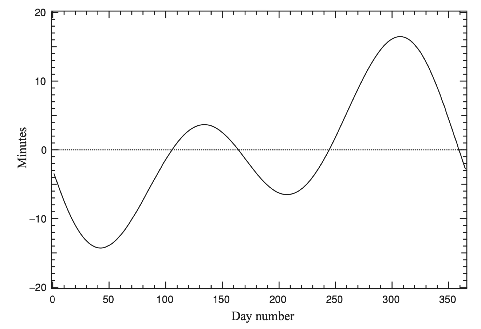
Source: Observational Astronomy, Birney et al. (2nd ed.)

These days the mean solar time is defined based on the position of far away sources using very long baseline interferometry, and as such a mean solar day is 24.0000006 hours (based on the SI definition of a second).

The solar mean time needs to be measured with respect to a given location on Earth, which for historical reason is chosen to the the Greenwich meridian (and as such called the Greenwich Mean Time or GMT, also often referred as Universal Time or UT). The time at a given location is then defined as the difference between the local mean solar time and the GMT based on the latitude of the place

\[ {\rm local mean time} = {\rm GMT} - {\rm longitude} \]

Dynamical time

The mean solar time is not a perfect measure of time. The rotation of the Earth is not constant and is affected by many factors, such as the gravitational pull of the Moon and the Sun, the tides, and the motion of the Earth’s crust. To account for these variations we need to define a new time scale, called dynamical time. Dynamical time has had multiple iterations over the years, from the original Ephemeris Time or ET to the Terrestrial Dynamical Time (TDT) or the current Terrestrial Time (TT). In all cases the dynamical time unit is the SI second. Dynamical time definitions are complex but they are designed to be free of the variations that affect the mean solar time.

Starting in 1970 a new time, the International Atomic Time (TAI) was introduced based on the combined measurements of over 450 atomic clocks distributed around the world. At the time of its inception TAI was defined to be (and remains) \(\rm TAI=TT-32.184\,s\).

Universal Time (UT or GMT) differs from TT or TAI by a factor \(\Delta T\) such that \(UT=TT - \Delta T\). The value of \(\Delta T\) cannot be predicted over a long period of time as it depends on precise measurements of the Earth’s Orientation Parameter, which are released by the International Earth Rotation and Reference Systems Service (in reality IERS releases the value of DUT1, a closely related concept). The following image shows the variation of \(\Delta T\) over the years.

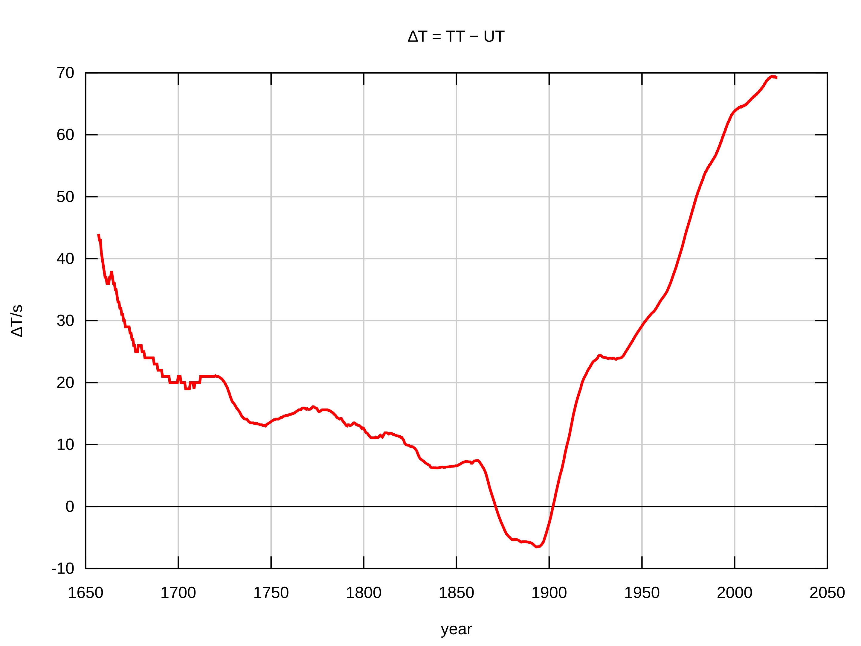
Source: Wikipedia

Since \(\Delta T\) is a complicated function of time, a new time was introduced the UTC or Coordinated Universal Time which has an offset with respect to TAI that is an integer number of seconds. Given that the rate of rotation of the Earth is continuously decreasing due to the influence of the Moon, UTC keeps diverging from TAI. By convention the difference between UTC and TAI is kept within 0.9 seconds by introducing leap seconds when necessary. Currently \(\rm UTC=TAI-37\,s\). UTC is commonly referred as the Civil Time and is the one used for most applications, including astronomical observations. It is important, however, to know what time scale we are using and whether it is the appropriate one for our purposes. Many astronomical libraries like astropy.time allow to convert between different time scales and are able to query the IERS Bulletins for updated values of the \(\Delta T\) or DUT1 parameters.

Sidereal time

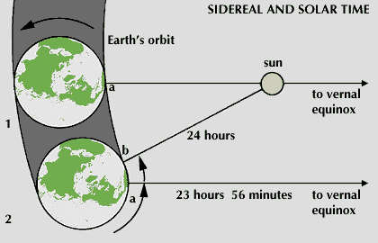
We have already introduced the concept of sidereal time, but let’s define it properly now. So far our definition of day and time has been based (albeit mostly from a historical perspective) in the successive transits of the Sun over the local median. However, if we were to do the same exercise using a distant star (say, Deneb, \(\alpha\ \rm Cyg\)), a precise watch would measure that the time between two consecutive transits is less than 24 hours (about 23 hours and 56 minutes).

The reason is that in the time between the two transits the Earth has moved a bit along its orbit around the Sun. Since the Earth completes an orbit around the Sun in approximately 365 days, the Earth moves a bit under a degree in one day, or about 4 minutes.

The sidereal time is defined based on the movement of the vernal equinox (or any fixed point on the celestial sphere). As with the apparent solar time, the sidereal time is affected by the ellipticity and inclination of the Earth’s orbit. Because of this a mean sidereal time (MST) is analogously defined. The mean sidereal time refers to the the time measured at the Greenwich meridian; the local sidereal time (LST) is related to the MST by the longitude of the location, \({\rm LST} = {\rm MST} - {\rm longitude}\).

Julian dates

The Julian date (JD) is a continuous count of days and fractions of days since the beginning of the Julian Period at 12h UT on January 1, 4713 BC. The Julian date is widely used in astronomy because it provides a simple and unambiguous way to specify dates and times. A Julian day is defined as 86,400 SI seconds, which is the same as a mean solar day. Note that Julian dates change at noon UT unlike civil time. For example, the Julian date corresponding to 12h UT on April 10th 2025 is 2460776.0.

Hint

Here is how to use astropy.time to determine the Julian date of a given time:

>>> from astropy.time import Time
>>> time = Time('2025-04-10 12:00:00', scale='utc')
>>> time.jd
2460776.0

We can also convert from a Julian date to a calendar date:

>>> time = Time(2460776.0, format='jd', scale='utc')
>>> time.iso
'2025-04-10 12:00:00.000'

A variation on the Julian date is the Modified Julian Date, which is defined as

\[ \rm MJD=JD-2400000.5 \]

Note that not only are MJDs more compact, they also start at midnight UT. Here is an MJD calendar for 2025.

Measuring light

Astronomy can be justifiably be described as the science of light. While other sciences are able to probe their subjects matters via a number of different means, astronomy mainly relies on the study of the light that astronomical sources emit, reflect, or otherwise process. Fortunately for us, electromagnetic radiation (light) encodes a wealth of information about the sources that emit it which we can study by means of photometry, spectroscopy, polarimetry, and other techniques.

The electromagnetic spectrum

Due to its wave-particle duality, the energy of a photon is related to its frequency or wavelength by the expression

\[ E = h \nu = \frac{hc}{\lambda} \]

where \(E\) is the energy of the photon, \(h\) is Planck’s constant (\(6.626 \times 10^{-34}\ \rm J\ s\)), \(\nu\) is the frequency of the photon, \(c\) is the speed of light in vacuum, and \(\lambda\) is the wavelength of the photon. Also note that

\[\begin{split} d\nu=d\lambda\cdot\dfrac{c}{\lambda^2}\\ \dfrac{d\nu}{\nu}=\dfrac{d\lambda}{\lambda} \end{split}\]

For convenience we often refer to the different parts of the spectrum by their wavelength ranges. While there is no strict definition the following ranges are commonly used:

Name	Wavelength
Gamma	0.1-10 \(\unicode{x212B}\)
X-ray	10-100 \(\unicode{x212B}\)
Far UV	100-1000 \(\unicode{x212B}\)
Near UV	1000-3500 \(\unicode{x212B}\)
Optical	3500-10000 \(\unicode{x212B}\)
Near IR	1-10 \(\rm \mu m\)
Mid IR	10-100 \(\rm \mu m\)
Far IR	100-1000 \(\rm \mu m\)
Microwave	1-100 \(\rm mm\)
Radio	> 0.1 m

As you can see, the units we typically use for for wavelength change depending on the type of radiation we are studying. Wavelength and frequency are related as \(\nu=c/\lambda\). Traditionally astronomers have used wavelength units for optical and infrared radiation, while radio astronomers use frequency units. In the case of X-ray and gamma-ray astronomy, both units are used.

Astronomers have many ways to quantify the amount of electromagnetic radiation emitted by an object. We can defined the specific intensity \(I_\nu\) (sometime called radiance) as the energy emitted by a surface per unit of area per unit of time per unit of frequency (or wavelength) and per unit of solid angle. The units of specific intensity are watts per steradian per square metre per hertz (or, in CGS, ergs per square centimetre per steradian per hertz per second). For an angle \(\theta\) that is measured from the normal to the surface

\[ I_\nu=\dfrac{dE}{\cos\theta dA\,dt\,d\nu\,d\Omega} \]

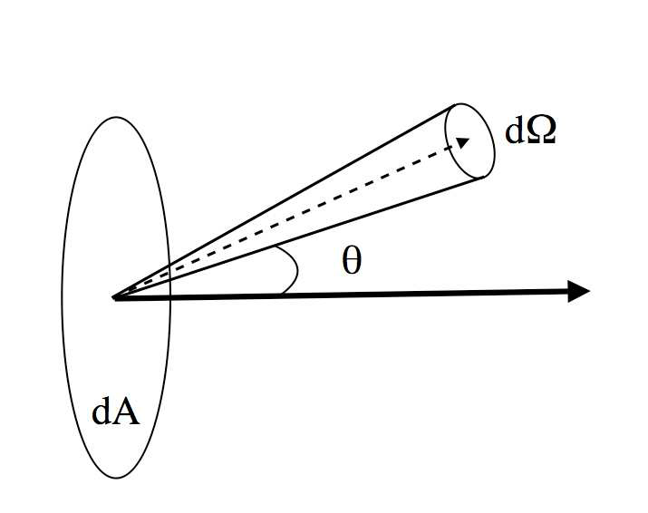
and \(I_\lambda=c/\lambda^2 I_\nu\).

The monochromatic flux (also called brightness or irradiance) is the amount of energy that passes through a unit surface from all directions

\[ F_\nu=\int I_\nu \cos\theta d\Omega \]

where we can often assume \(\cos\theta\approx 1\) since our detectors only collect photons from a small solid angle perpendicular to its surface.

Note that as with the specific intensity, the monochromatic flux (sometimes called flux density) is defined per unit of frequency or wavelength. We can integrate over the entire wavelength range to get the total flux \(F\).

The luminosity is the total amount of energy emitted by a source per unit of time and is related to the total flux by the distance to the source

\[ L = 4\pi d^2 F \]

Note

Astronomers normally measure flux for unresolved sources (point source, for example stars) and specific intensity (often called surface brightness in this context) for extended sources (like galaxies).

While some types of detectors (for example bolometers) are able to measure the spectrum of the light (the specific intensity), most detectors measure the number of photons received over time. Because of this we need to define the photon flux \(F_{{\rm photon}}\) as

\[ F_{{\rm photon}}=\int F_\lambda\dfrac{\lambda}{hc}d\lambda \]

Magnitudes

The quantities defined in the previous section express the amount of light emitted by a source. Astronomers, however, tend to use a different system to measure flux (brightness): magnitudes. The magnitude system was first defined by the Greek astronomer Hipparchus in the 2nd century BC. In this system start of magnitude 1 are the first ones visible to the naked eye just after sunset, while the faintest starts visible at the end of the twilight are of magnitude 6. Intermediate magnitudes were defined by dividing the twilight in equal parts. The magnitude system remained in used for many centuries and, while imprecise, it was not until the advent of photography and detectors that could measure light more quantitatively that the system was redefined.

The modern magnitude system takes into account that the human eye responds to stimuli in an approximately logarithmic way. From that, the difference in apparent magnitude between two sources is defined as proportional to the logarithm of the ratio of their fluxes:

\[ m_1 - m_2 \propto \log_{10}\left( \dfrac{F_1}{F_2} \right) \]

In the 19th century the English astronomer Pogson further refined this definition by requiring a start of magnitude 6 to be 100 times fainter than one of magnitude 1. This is equivalent to

\[ m_1 - m_2 = -2.5 \log_{10}\left( \dfrac{F_1}{F_2} \right) \]

and also equivalent to saying that a star of magnitude 2 is \(100^{1/5}\approx2.512\) times fainter than a star of magnitude 1. Note the minus sign that is encodes the fact that larger magnitudes mean fainter sources. Apparent magnitudes defined this way are called Pogson magnitudes.

Important

Pogson magnitudes are always defined using photon fluxes.

Apparent magnitudes are defined for a given passband or wavelength range (more on this later). Bolometric magnitudes account for the electromagnetic flux received from a source in all wavelengths. The difference between the apparent magnitude in a bandpass \(X\) and the total bolometric magnitude is called the bolometric correction, \({\rm BC}_X\) and is defined as

\[ {\rm BC}_X = m_{\rm bol} - m_X \]

In practice bolometric magnitudes are very difficult to measure and the bolometric correction is usually estimated from the spectral energy distribution (SED) of the source, which are in turn determined from models for a given astronomical object (for example, for a start of a certain spectral type).

The absolute magnitude \(M\) is defined as the apparent magnitude of a source at a distance of 10 parsecs. It is related to the apparent magnitude \(m\) and the distance \(d\) (in parsecs) to the source by

\[ m - M = 5 \log_{10} d - 5 \]

Finally, the absolute bolometric magnitude is directly related to the luminosity of a source using the solar luminosity as a reference:

\[ M_{\rm bol} = -2.5 \log_{10} \left( \dfrac{L}{L_\odot} \right) + 4.74 \]

where \(L_\odot\) is the luminosity of the Sun. The absolute bolometric magnitude is a measure of the total energy emitted by a source and is independent of distance.

Photometric systems

So far all the the apparent magnitudes we have defined have been in reference to another magnitude, that is to the ratio of their fluxes. We can do

\[ m - m_0 = -2.5 \log_{10}\left( \dfrac{F}{F_0} \right) m = -2.5 \log_{10} F + C(\lambda) \]

where \(C(\lambda)\) is called a zero-point and refers to the flux that corresponds to a magnitude of 0 for a given wavelength. The choice and characterisation of \(C(\lambda)\) is what define a photometric system.

Historically most photometric systems where defined so that the zero-point corresponds to the flux of Vega at each wavelength, and as such are called VEGAMAG systems. Later the average spectrum of a group of A0V stars such as Vega was used. Vega was used as a reference for two reasons: it’s one of the brightest stars on the sky and A-type stars have relatively smooth, well understood spectra.

One of the most common photometric systems, the UBVRI system or Johnson can be defined for each bandpass as

\[ m_{UBVRI} = -2.5 \log_{10}\dfrac{\int_{UBVRI}F_{UBVRI}\lambda d\lambda}{\int_{UBVRI}F_{UBVRI}({\rm Vega})\lambda d\lambda} \]

where the integrals are over the bandpass of the filter and the \(\lambda\) factor is included to convert from flux to photon flux.

A conceptually different photometric system is the AB magnitude system. Here we assume a constant zero-point flux \(F_{0,\nu}=3631\, {\rm Jy}\) which is the flux density of Vega at \(5500\,\unicode{x212B}\) in Jankys. With this

\[ m_{AB}=-2.5\log_{10} F_\nu-48.6 \]

when \(F_\nu\) is in Jy. Normally we defined an AB magnitude for a certain filter bandpass so that

\[ m_{AB}=-2.5\log_{10}\dfrac{\int (F_\nu / \nu) d\nu}{\int (F_{0,\nu}/\nu) d\nu} \]

where again the \(1/\nu\) factor is included to convert from flux to photon flux.

The STMAG zero-point system makes similar assumptions to the AB system but for a constant flux per unit of wavelength and was developed primarily for the Hubble Space Telescope bandpasses.

Why are AB and STMAG systems not the one primarily used? While much more simpler to define, the AB and STMAG systems are not based on a real source (there are no sources with a constant flux density) and as such they are more difficult to calibrate. However the most common modern photometric systems are either based on the AB system or have been cross-calibrated and allow for a direct comparison with it.

Colours

The colour index or just colour is the difference between two magnitudes in different bandpasses. In this case the colour corresponds to the ratio of fluxes (a concept that is closely related to the usual definition of “colour”). For a VEGAMAG system, the colour gives the ratio of the fluxes relative to the ration of the fluxes of an A0V star.

Surface brightness

So far we have implicitly discussed the brightness of unresolved point sources. For a resolved sources like a galaxy or a nebula we can define an equivalent concept, the surface brightness, \(S_X\) (for a bandpass \(X\)) can be defined as the magnitude equivalent to the average flux per square arcsecond. If the object in question subtends an area \(A\) an \(\rm arcsec^2\) then

\[ S_X=-2.5\log_{10}\left(\dfrac{F_X}{A}\right)= -2.5\log_{10} F_X + 2.5\log_{10} A = m_X+2.5\log_{10} A \]

Filters

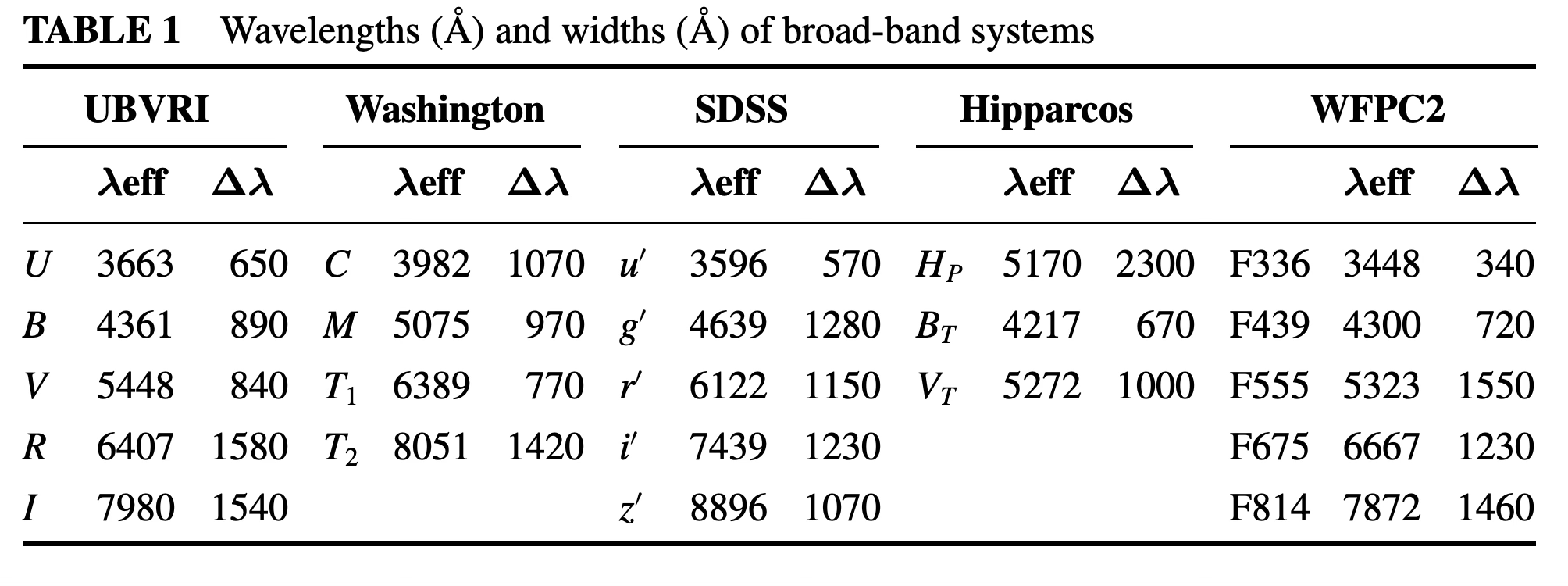
Photometric systems are usually defined for a set of well-defined filters, each one letting pass only a certain range of wavelengths, and with a known transmission curve. The following figure shoes the transmission curves of several common photometric systems/filter sets. Often the filters (e.g., the SDSS system) were developed for a specific telescope and project but have since become widely used.

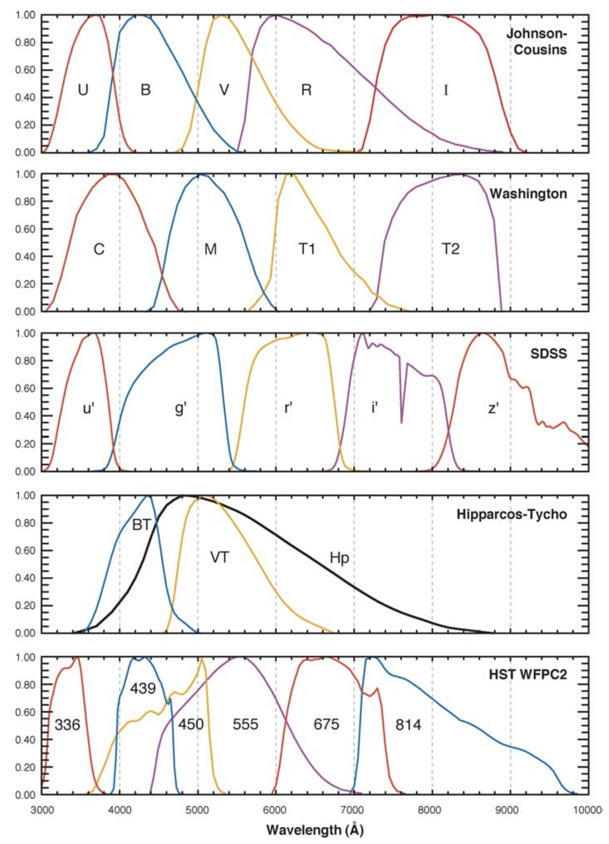
Photometric systems are often defined in terms of their effective central wavelength and the equivalent width of the filter. The equivalent width is defined as that of a rectangular filter with 100% transmission centred around the effective wavelength.

These filters are usually called “broadband” because they have non-zero transmission over a wide range of wavelengths (hundreds or thousands of angstroms). There are also “narrow-band” filters, which have a much narrower transmission range (typically 10-100 \(\unicode{x212B}\)) and are used to isolate specific spectral lines. Typical narrow-band filters are H\(\alpha\) [OII], [OIII], [SII], etc. For extragalactic targets the recession velocity of the source needs to be taken into account as the emission line of interest may have been red- or blue-shifted. Because of that narrow-band filters are often produced in sets to cover a range of central wavelengths.

Optics and telescopes

While for millennia we relied only on our eyes to observe the sky, the development of optics, and in particular of telescopes, soon revolutionised astronomy. Telescopes allow us to collect more light and to resolve finer details than the human eye alone. Here we will very briefly discuss some of the basic concepts surrounding optics and telescopes.

Basic principles

The basic principle of classic optics is Snell’s law, which relates the angles of incidence and refraction of light passing through the boundary between two different media.

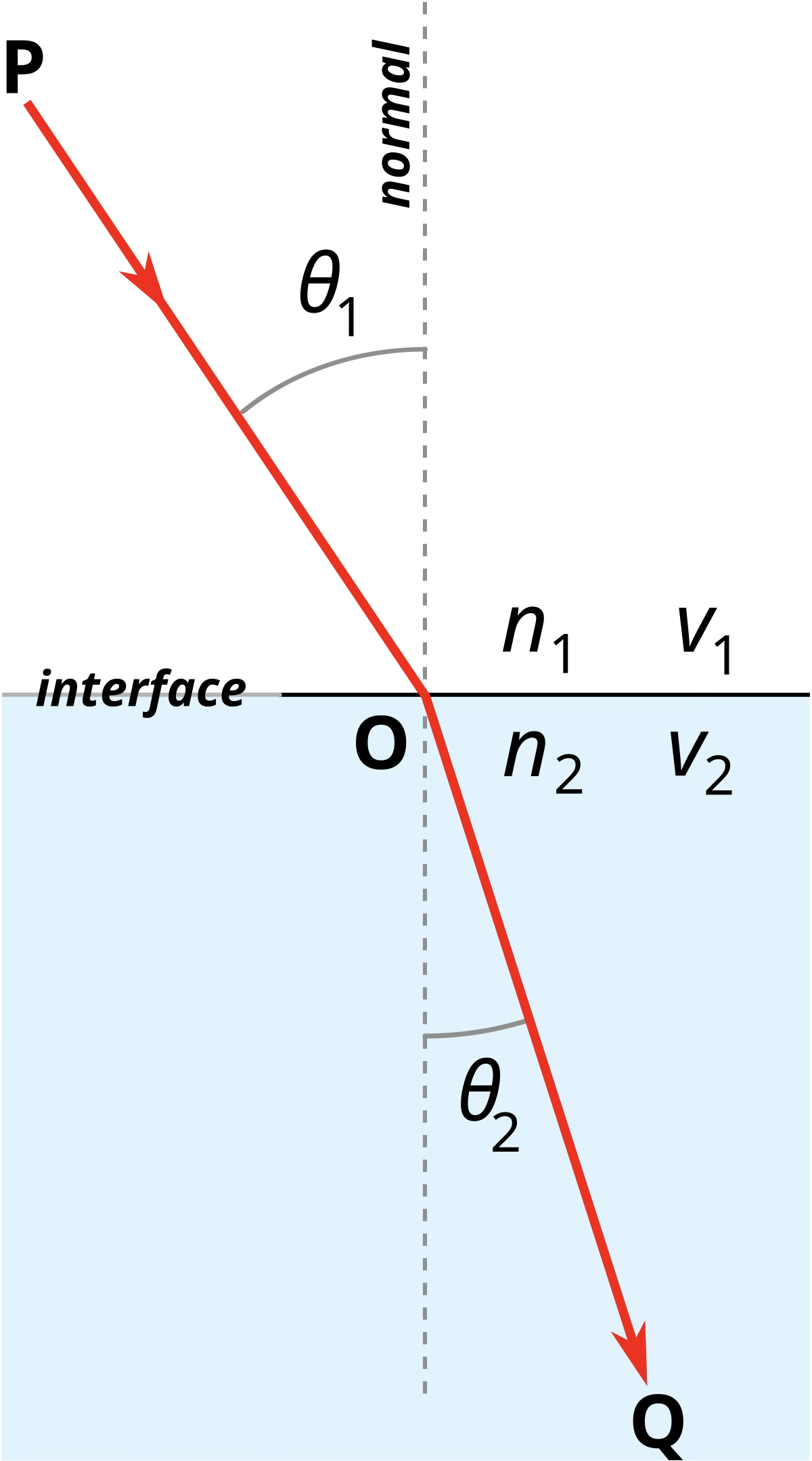
Source: Wikipedia

Snell’s law can be expressed as

\[ n\sin i = n^\prime \sin i^\prime \]

where \(n\) and \(n^\prime\) are the indices of refraction of the two media, \(i\) is the angle of incidence, and \(i^\prime\) is the angle of refraction. The index of refraction is defined as the ratio between the speed of light in vacuum and the speed of light in the medium. The angles are measured with respect to the normal to the surface.

Snell’s law can also be used to describe the reflection of light. In this case \(n=n^\prime\) and \(i=-i^\prime\) (the angle of incidence is equal to the angle of reflection).

Snell’s law is a special case of Fermat’s principle, which states that light travelling between two points will follow the path that can be travelled in the least time.

Paraxial approximation and thin lenses

The paraxial approximation in optics assumes that the angles of incidence and refraction on a surface as small, so that \(i\ll1\) and \(\sin i\approx i\). In this regime many of the equations of optics can be simplified and the behaviour of light can be described using simple geometric optics. We can also disregard most aberrations while we are close to the optical axis. The paraxial approximation is usually combined with the thin lens approximation, which assumes that the thickness of the lens is small compared to its focal length (which we’ll describe in a second). In this case we can treat the lens as a single surface. For now we will also ignore the effects of diffraction, which is usually ok when the aperture of the lens is very large compared to the wavelength of the light.

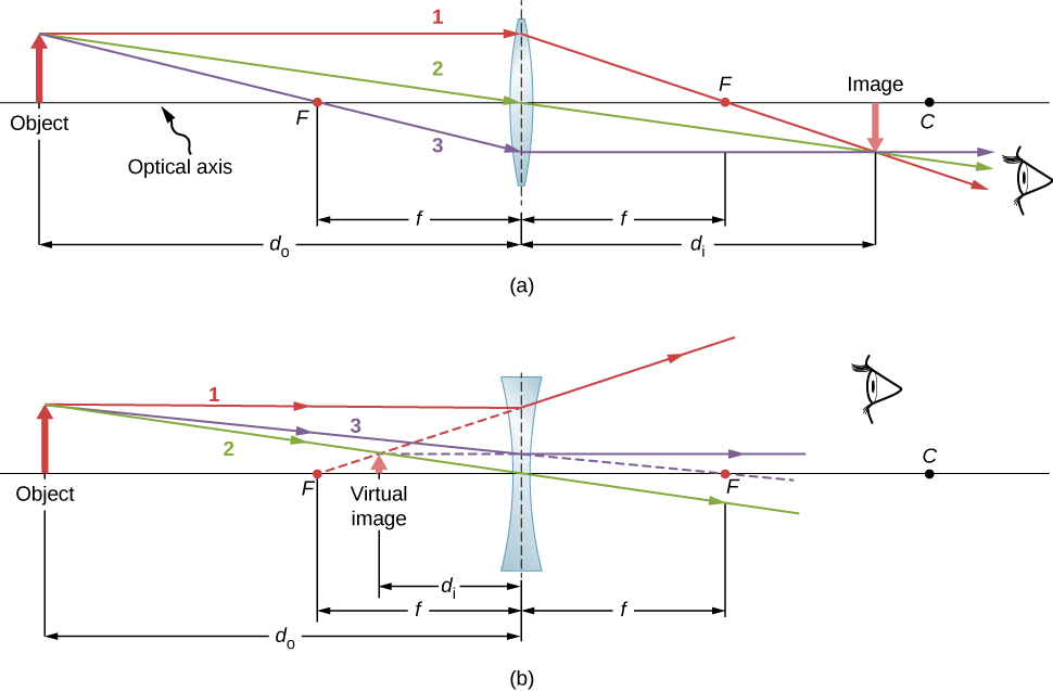
Let’s consider two cases of thin lenses: one with a convex surface (top) and one with a concave surface (bottom).

First we’ll define a few concepts:

• A meridional ray is one that is limited to the plane formed by the optical axis of the system and the point on which the ray originated. All rays of interest in this section are meridional rays.

• The chief ray or principal ray is one that starts at the edge of the object that emits the ray and passes through the centre of the optical element (in reality it’s the ray that passes through the centre of the aperture stop, but as we’ll see that usually means the same thing). If the lens is symmetric —both surfaces have the same but opposite curvature— the chief ray passes through the centre of the lens without deflection (really the light “bends” twice, once at each surface, but the net effect is no deflection).

• The distance between the lens to the object (\(d_o\)) and to the image (\(d_i\)) are called the conjugate distances. Note that in case a) the \(d_i>0\) but \(d_o<0\) while in case b) both distances are negative.

• The point where a ray that is parallel to the optical axis intersects the optical axis is called the focal point (\(F\)) and the distance between the lens and the focal point is called the focal length (\(f\)). The focal length is positive for a converging lens and negative for a diverging lens. For an object at an infinite distance (as is the case, in excellent approximation, for astronomical sources) the focal point defines the point where all the rays coming from the object converge.

• The image is the point where the optical rays converge after passing through the lens. The image is real if the rays actually converge at a point and virtual if they only appear to converge at a point (i.e., the rays diverge after passing through the lens). In a converging lens the image is real (the rays actually converge) while in a diverging lens the image is virtual (the rays diverge after passing through the lens) and located in the place where the back-propagation of the rays converge. However, whether an image is real or virtual depends on the position of the object with respect to the lens. For example, if we place an object at a distance \(d_o\) from a converging lens, the image will be real if \(d_o>f\) and virtual if \(d_o<f\). The opposite is true for diverging lenses.

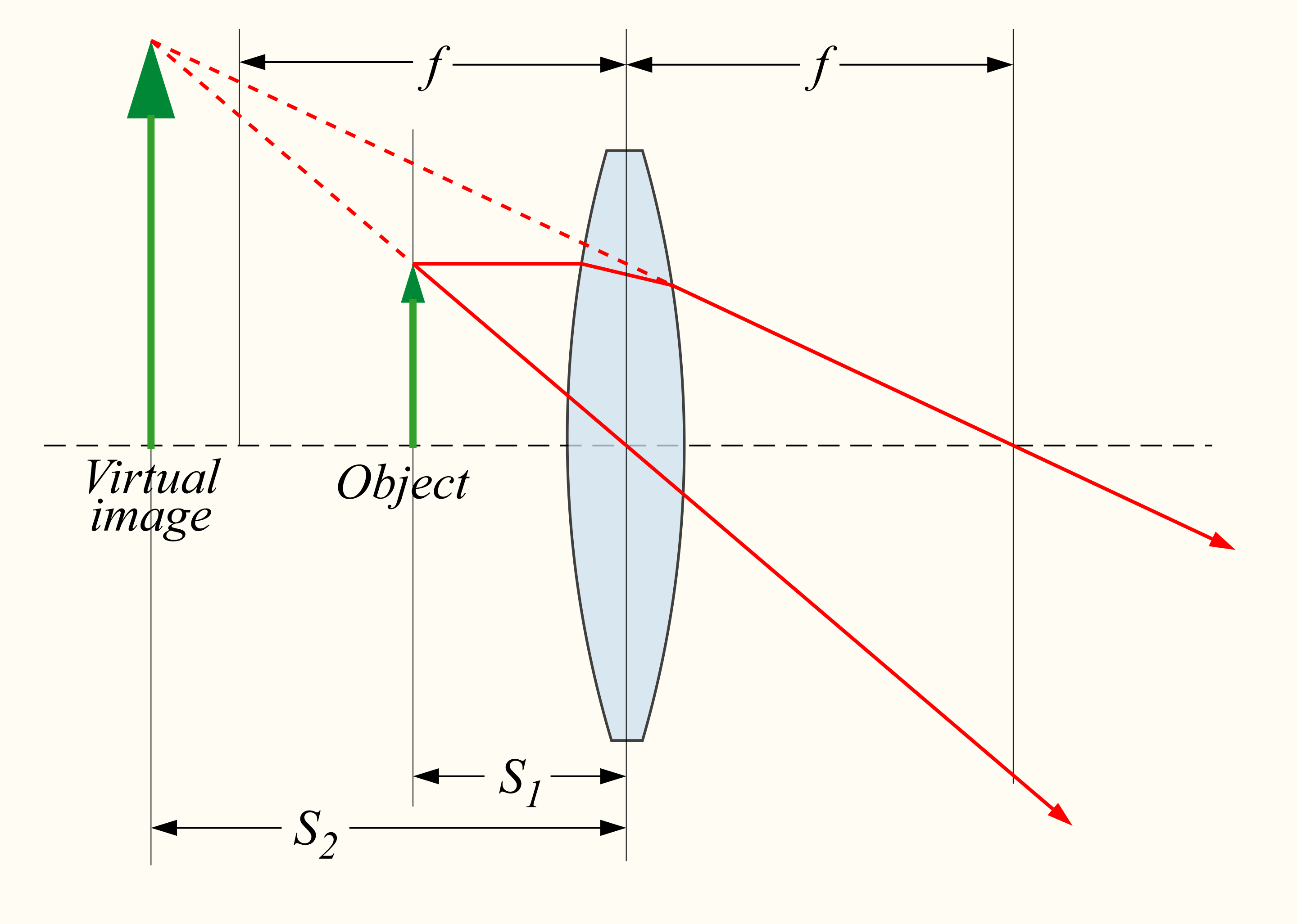
A converging lens with a virtual image. Note that the object is located at a distance of the lens that is smaller than the focal length. Source: Wikipedia

From simple geometric relationships (see, for example Schroeder, Astronomical Optics, Ch. 2) we can derive the following expression for a single refracting surface:

\[ \dfrac{n^\prime}{d_i}-\dfrac{n}{d_o}=\dfrac{n^\prime-n}{R} \]

where \(R\) is the radius of curvature of the surface, \(n\) is the index of refraction of the medium where the object is located, and \(n^\prime\) is the index of refraction of the lens. The right side of this equation is called the power of the lens and is independent of the positions of the object and image. The power defines the ability of the lens to converge or diverge light. The power of the lens is related to the focal length by

\[ P \equiv \dfrac{(n^\prime-n)}{R}=\dfrac{n}{f}=\dfrac{n^\prime}{f^\prime} \]

However, lenses are formed by two surfaces. In this case we can write the power as

\[ P=\dfrac{1}{f^\prime}=(n^\prime-1)\left(\dfrac{1}{R_1}-\dfrac{1}{R_2}\right) \]

where \(1/f^\prime=1/f_1+1/f_2\) is the equivalent focal length of the system and \(R_1\) and \(R_2\) are the radii of curvature of the two surfaces. Here we assume that the lens is thin and that the medium in which it is located has \(n^\prime\approx1\) (as is the case for air). \(n^\prime\) is the index of refraction of the lens material.

For the case of reflection we have a single surface. In this situation we can write that

\[ \dfrac{1}{d_i}+\dfrac{1}{d_o}=\dfrac{2}{R} \]

and the focal length of a mirror is given by \(f=R/2\).

Additionally, we can define the focal ratio or f-number of a lens or mirror as the focal length divided by the diameter of the aperture. In astronomy, for a fixed aperture, the f-number is a measure of how fast the beam of light is converging. Because of this, optical systems with a small f-number are called fast and those with a large f-number are called slow.

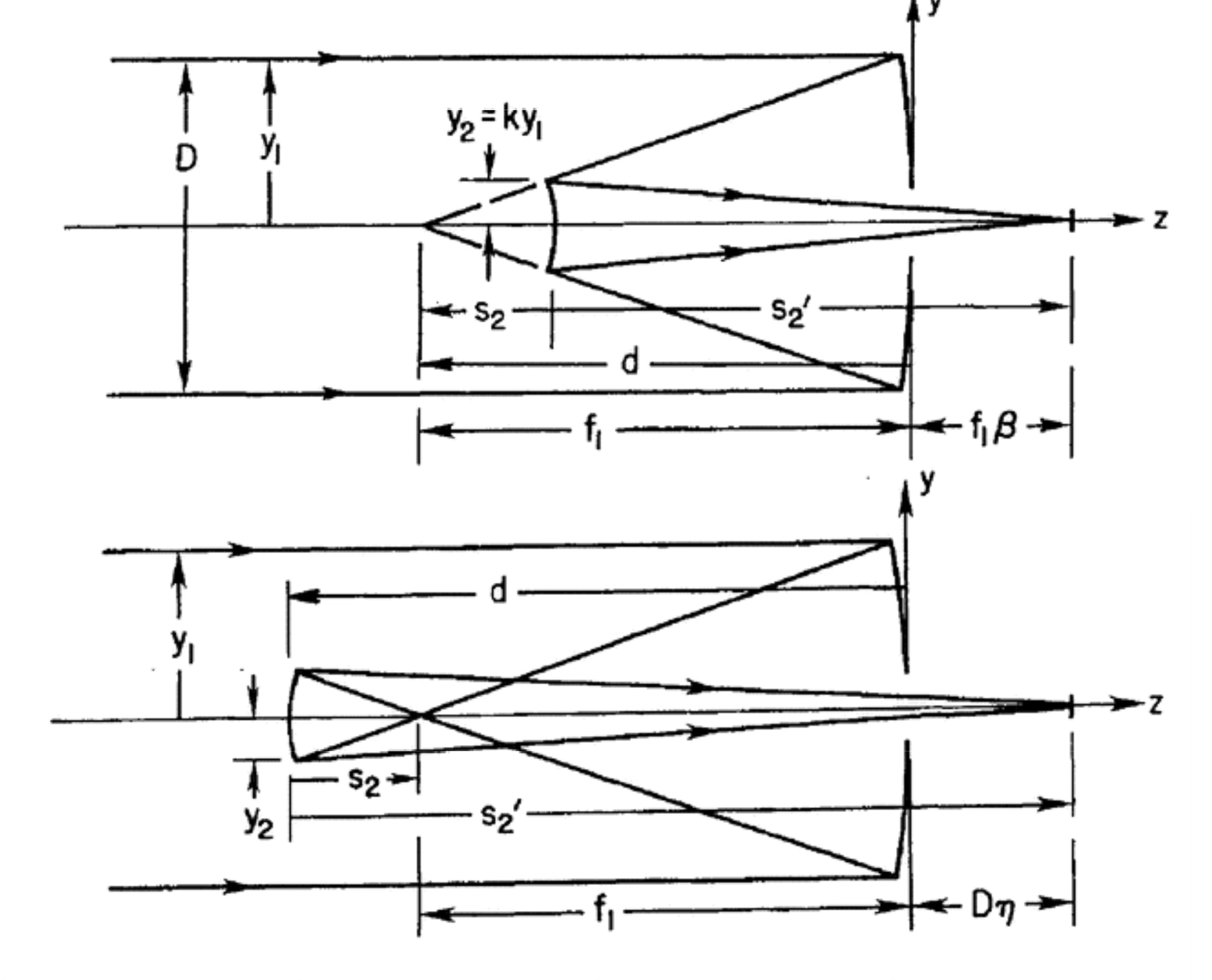
Another important concept is that of the magnification of an optical system. The magnification is defined as the ratio between the size of the image and the size of the object.

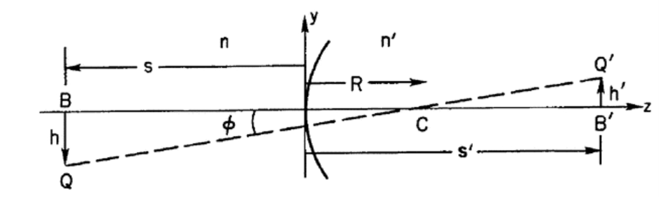
Source: Schroeder, Astronomical Optics

For a lens, the magnification is given by

\[ M=\dfrac{h^\prime}{h}=\dfrac{s^\prime-R}{s-R}=\dfrac{ns^\prime}{ns} \]

(note that if the magnification is negative the image is inverted).

However, for the most usual case in astronomy, the object is at an infinite distance, \(s=\infty\), and the magnification is zero (this does not mean that a telescope cannot magnify an object at an infinite distance, it just means that the image is formed at the focal plane of the lens, but other optical elements placed before or after the focus can magnify the image). Instead, a more relevant concept is that of the scale, which is the smallest separation between two points that can be resolved by the optical system. The scale is defined as

\[ S=\dfrac{1}{f}=\dfrac{206265}{f\,[\rm mm]}\,[\rm arcsec/mm] \]

Finally, let’s consider the case of two plane-parallel plates of glass with thickness \(d\) and index of refraction \(n\). This optical element does not change the magnification of a system, but it introduces a shift in the image position. The shift is given by

\[ \Delta = d\left[1-\left(\dfrac{1}{n}\right)\right] \]

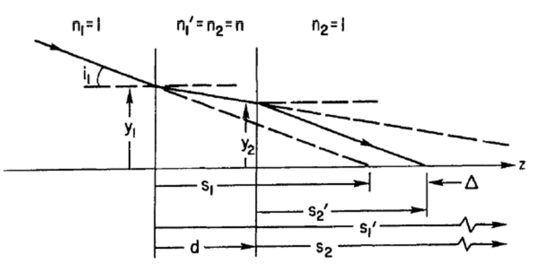
Source: Schroeder, Astronomical Optics

Apertures and pupils

We will quickly introduce the concept of pupil and aperture. These are important concepts that play a significant role in the design of optical systems.

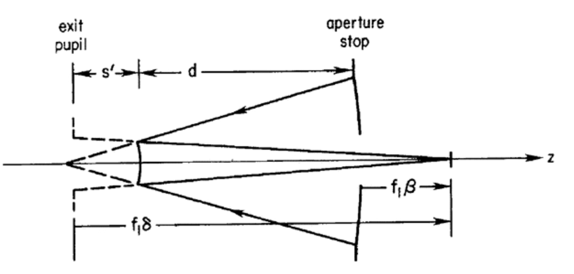
Source: Schroeder, Astronomical Optics

• Pupil: location where rays from all field angles fill the same aperture.

• Aperture stop: determines the amount of light reaching an image. This is usually the primary mirror or objective lens but in some cases, such as infrared telescopes, it can be a secondary mirror or a filter.

• Field stop: determines the angular size of the field. This is usually the detector but, for a large enough detector, it could be the secondary.

• Entrance pupil: the image of aperture stop as seen through any optical elements that precede it. Usually the entrance pupil is the same as the aperture stop. The entrance pupil is important to determine the field of view of the system and is the best location to place baffles to block stray light.

• Exit pupil: image of the aperture stop formed by all subsequent optical elements. The exit pupil is important to determine the system aberration and to measure the light wavefront.

Telescopes

A telescope is an optical system designed to collect light from a distant source (i.e., one that we can consider at infinite distance for optical purposes). The simplest telescopes, first built in the early 17th century, consisted of just an objective lens and an eyepiece. The objective lens is usually a converging element and determines the amount of light from the source that we can collect, while the eyepiece can be either converging (if located after the focal point of the objective) or diverging (if located before).

While simple, refracting telescopes have a number of problems, such as chromatic aberration (which we’ll discuss shortly). Constructing large refracting telescopes is also difficult, an in practice the largest refracting telescope, the Yerkes Observatory telescope, is only slightly over 1 metre in diameter.

The solution to these problem was found in 1666 by Isaac Newton (although the concept of magnifying images using curved mirrors goes back at least to the 11th century). The objective lens can be replaced by a concave mirror (usually parabolic) which focuses the light on the eyepiece. The following image shows simplified designs for the most common types of telescopes.

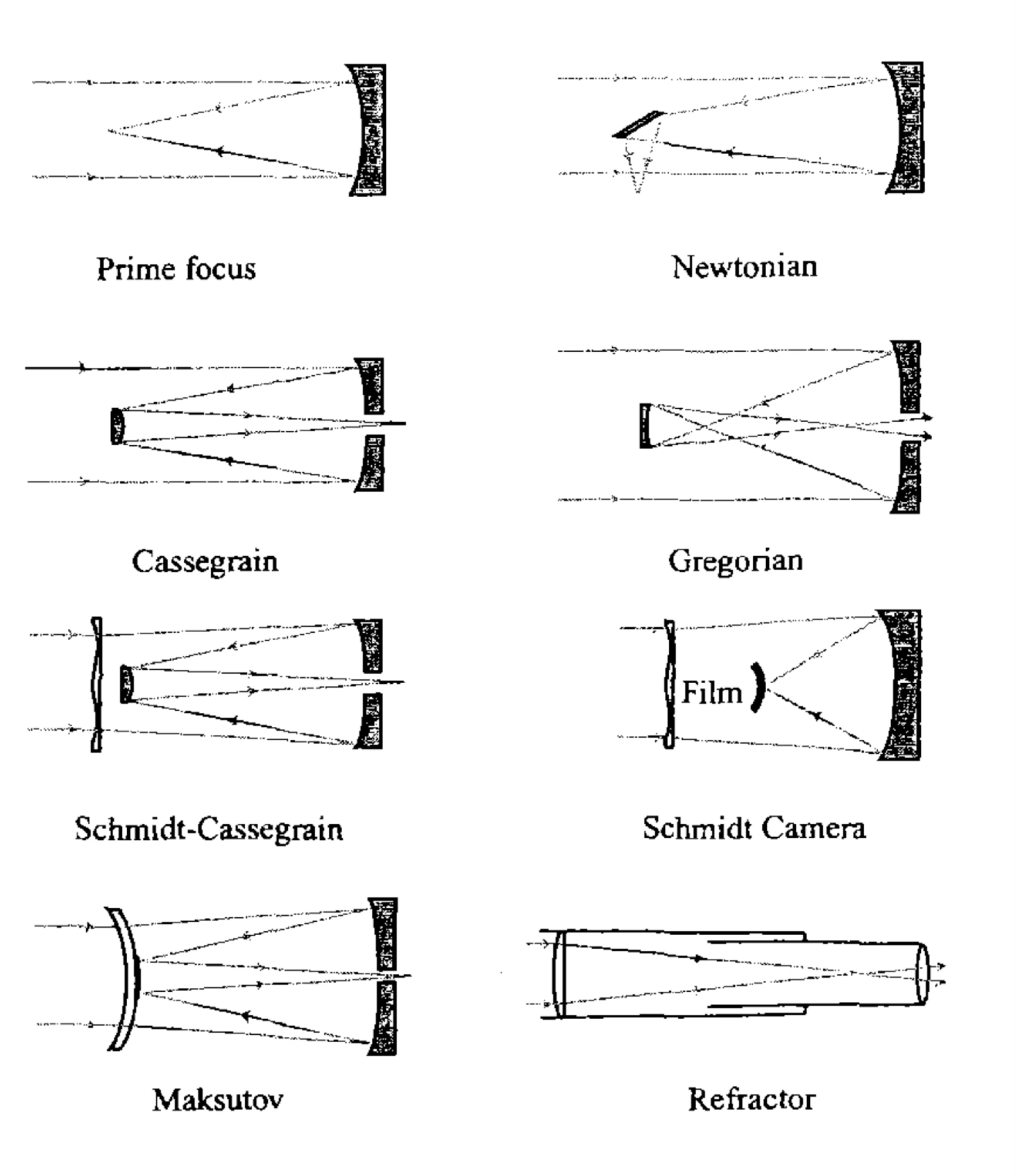
Source: Observational Astronomy, Birney et al.

Most reflecting telescopes consist of two mirrors: a large primary mirror that collects the light, and a smaller secondary mirror that reflects it to a focus. The Newtonian telescope uses a flat secondary that just moves the focus to the side of the telescope, where an eyepiece or camera can be placed. The Cassegrain telescope uses a parabolic primary and a convex hyperbolic secondary placed before the focus of the primary. Another common design is the Gregorian telescope, which replaces the secondary with a concave ellipsoid.

Cassegrain (top) and Gregorian (bottom) telescope designs. Source: Schroeder, Astronomical Optics

In some cases, such as the Schmidt-Cassegrain or the Maksutov telescopes, an spherical mirror is used for ease of manufacturing. These telescopes suffer from significant spherical aberration which is compensated by using a special corrector plate in front of the primary mirror. Amateur telescopes often use this design because of its compactness and relatively lower price, but constructing corrector plates for large apertures soon becomes prohibitively expensive.

Most modern telescopes use a Ritchey–Chrétien design, with hyperbolic primary and secondary mirrors. This design removes most low-order aberrations at the cost of being more difficult to manufacture. Additional optical defects are usually corrected by using a set of corrector lenses near the focal plane. Placing the corrector near the focus allows for it to be smaller and lighter, but since the beam of light is converging, the corrector is usually harder to design and manufacture.

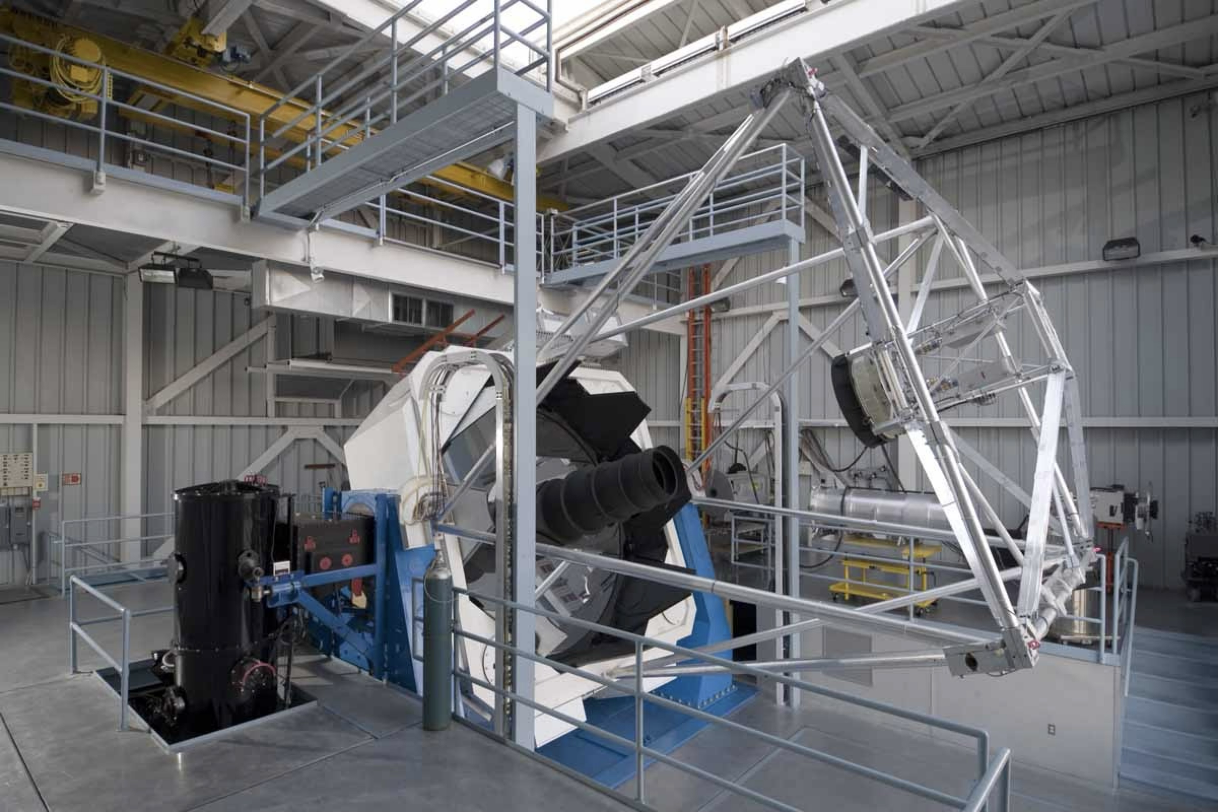
The 3.5-metre telescope at the Apache Point Observatory. The telescope uses a Ritchey–Chrétien design. The secondary mirror can be seen at the top of the telescope, supported by the truss structure. The Cassegrain focus is located behind the primary mirror (which has a hole to allow the light to pass). Alternative foci can be created by placing a third, flat mirror, just behind the primary. This mirror moves the focus to one or more Nasmyth foci located at the sides of the telescope. The advantage of the Nasmyth foci or “port” is that the instruments do not need to move with the telescope, which simplifies engineering and improves instrument stability. Source: Apache Point Observatory

Mounts

Telescopes need to be mounted on a structure that allows to point them to a desired location on the sky and, most importantly, to track that position as the Earth rotates. There are two main types of mounts: alt-azimuthal and equatorial.

The alt-azimuthal (or alt-az) mount has two axes of rotation, one that moves the telescope up and down (altitude) and another that moves it coplanar with the horizon (azimuth). Note that this are the same axes as the alt-az coordinates.

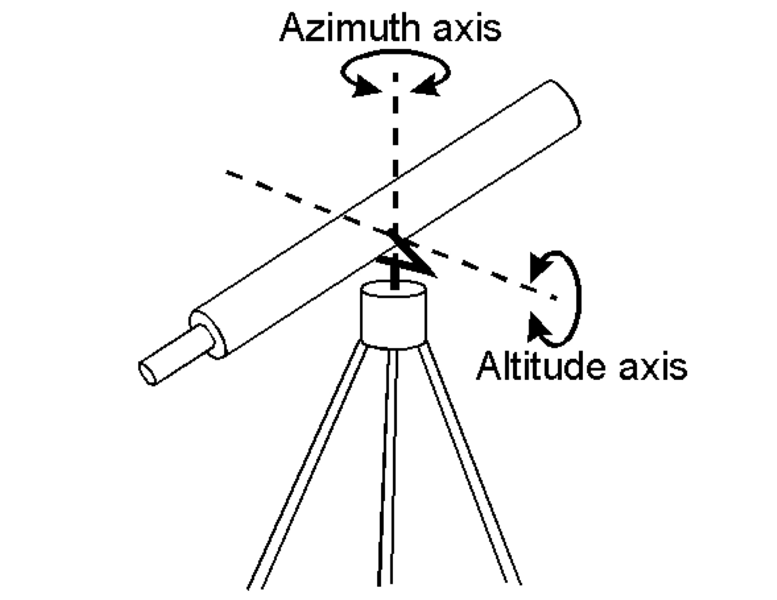
The advantage of the alt-az design is that is simple and that the centre of mass of the telescope is just above the mount, which makes it more stable. The disadvantage is that the telescope needs to be moved in two dimensions to track a source. Additionally, the even if we track a source on the sky by appropriately moving both axes, the field of view of the telescope will rotate. This is called field rotation and is caused by the fact that the field of view is not a single point. As the sky rotates, only the centre of the field of view is stationary, the rest of the field rotates around it. To compensate for this, the field needs to be rotated (or “de-rotated”) during the observation. This is done by a mechanism called the rotator, which depending on the telescope may move just the an optical element in the instrument, or rotate the entire back of the telescope.

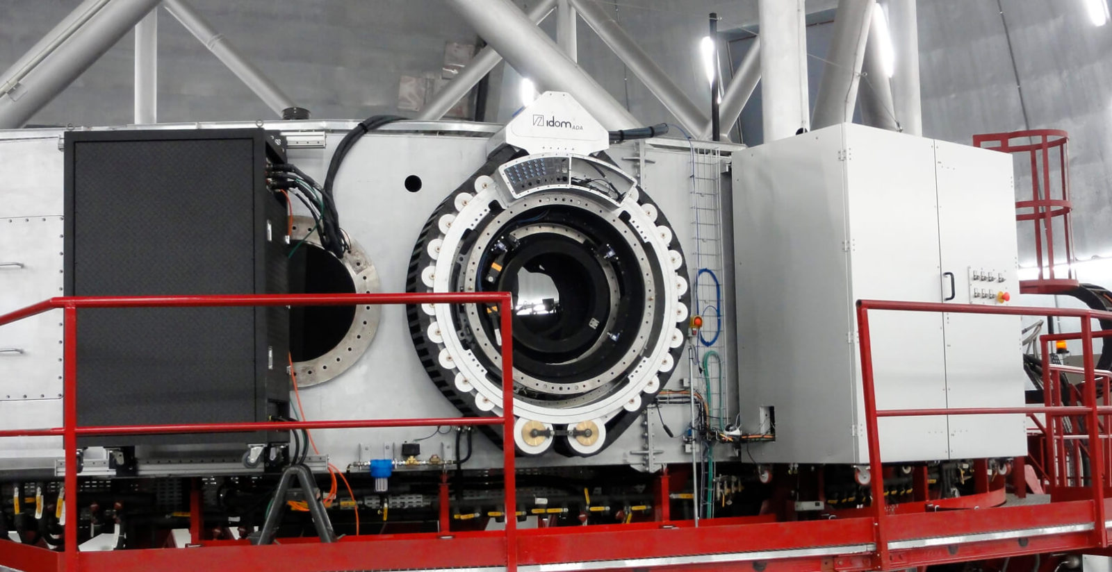
A rotator mechanism for the Gran Telescopio de Canarias (GTC). The rotator is located in one of the Nasmyth ports of the telescope and rotate any instrument attached to it. Note the corrector lenses at the centre of the corrector. Source: IDOM.

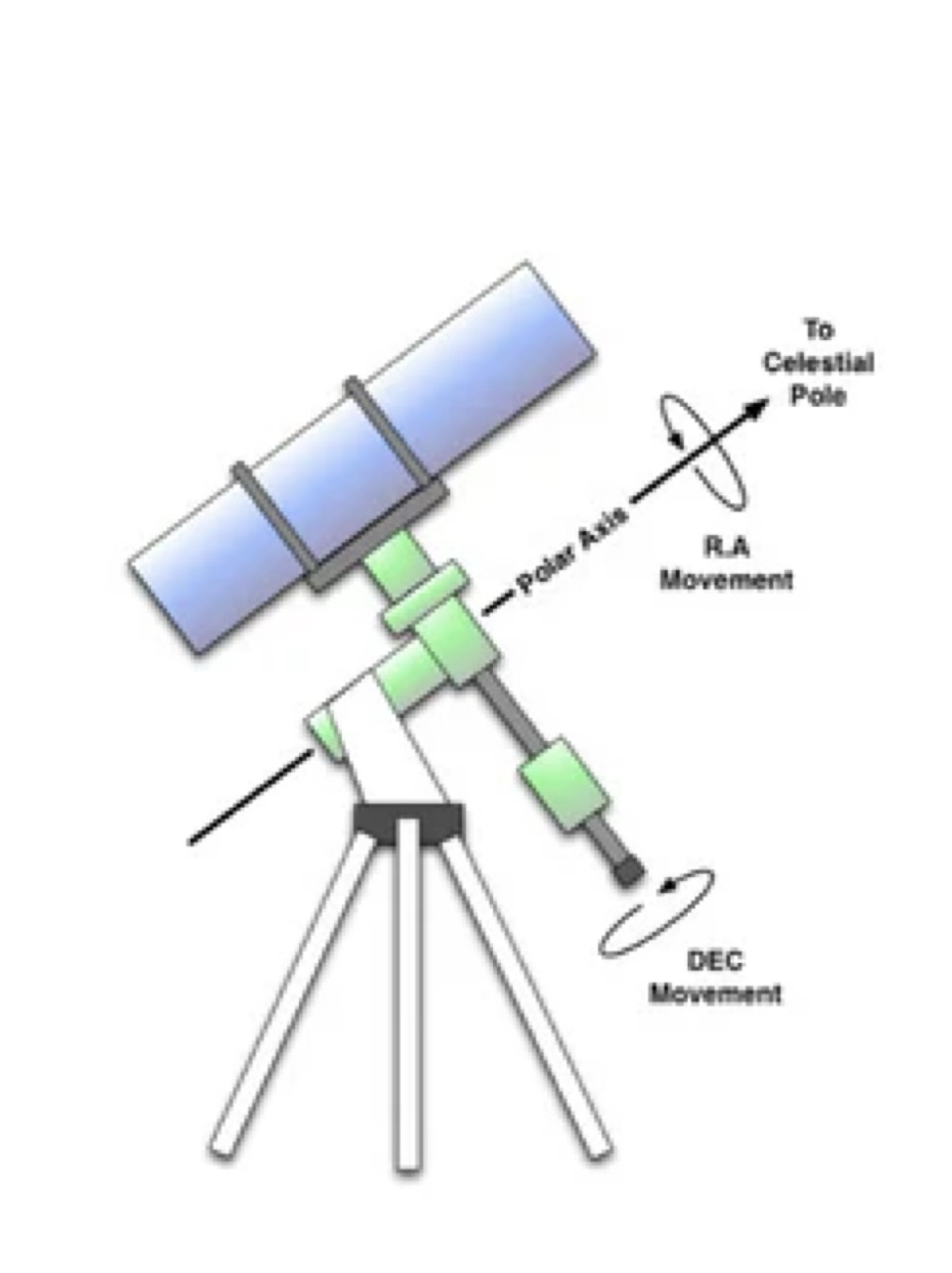
A solution to these problems is the use of an equatorial mount. In this case one of the axes of rotation (right ascension) is aligned with the Earth’s axis of rotation (i.e., points to the celestial pole). This means that we only need to move one axis to track a source on the sky. The other axis (declination) is used to point the telescope to a desired location on the sky.

The main disadvantage of the equatorial mount is that the weight of the telescope is often misaligned with the mount, which requires it to be over-engineered to avoid vibrations. In practice, an unless the polar alignment is perfect, the telescope will still need to be moved in two axes to track a source, although the contribution of the declination axis is usually small. Similarly, equatorial mounts are usually affected by a small amount of field rotation, which may or may not need to be corrected depending on the length of the observation, instrumentation, scale, etc.

Nowadays most large telescopes are build with alt-az mounts, and the problems of two-axis tracking and field rotation are solved by the use of guiding cameras and a closed-loop control system that continuously monitors the location of the telescope and adjust the position of all the axes.

Aberrations

So far we have limited ourselves to the paraxial and thing lens approximations. In reality, however, lenses and mirrors are not perfect. Aberrations arise when the image formed by an optical system is not a perfect representation of the object. There are many types of aberrations: chromatic, coma, spherical, … We will briefly discuss the most common ones below.

Aberrations can be avoided or compensated by taking into account Fermat’s principle: light travels between two points along the path that takes the least time. However, it is often not possible to derive a closed-form solution for the path of light rays in an optical system, and the behaviour of these systems needs to be studied using ray tracing and numerical methods.

Chromatic aberration

The simplest type of aberration is the chromatic aberration. This is caused by the fact that the index of refraction of a medium depends on the wavelength of the light passing through it. In practice this causes light of different wavelengths (colours) to be focused at different distances from the lens.

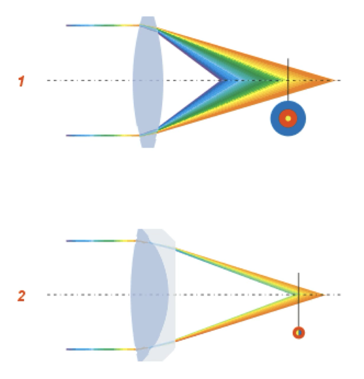
Chromatic aberration is much less prevalent in mirrors, although it is still present in some cases. In lenses this aberration can be reduced by using a combination of lenses made of different materials (called achromatic doublets or triplets). The complexity of these designs is one of the reasons why large refracting telescopes are so expensive to build. However, chromatic aberration and achromatic elements are important in other optical systems, such as cameras and spectrographs, which use lenses as part of their design.

Spherical aberration

Spherical aberration is caused by perfectly spherical lenses or mirrors. As we move aways from the optical axis and the paraxial regime, the rays of light are not focused at the same point. This results in a series of concentric rings of light, which is called a circle of confusion.

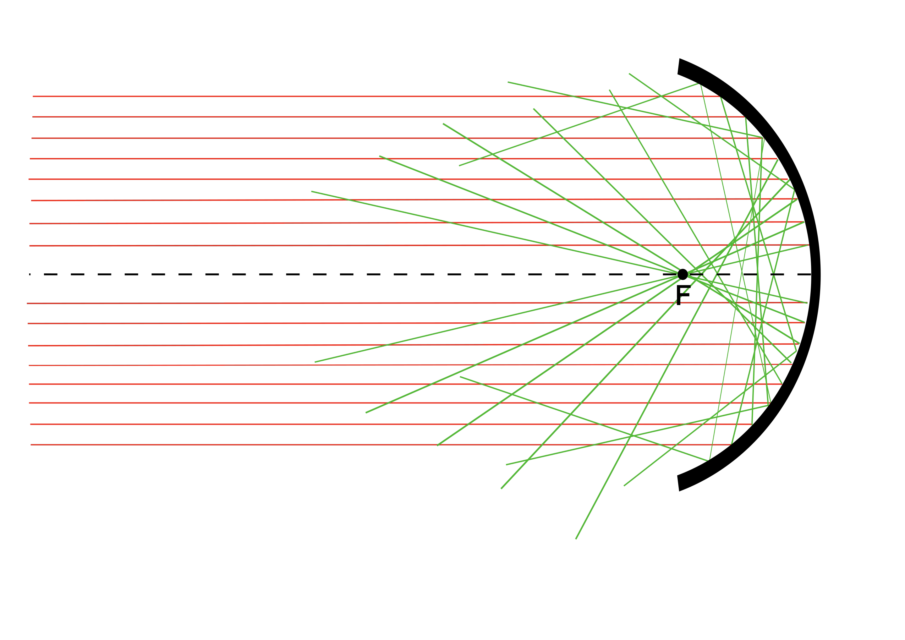
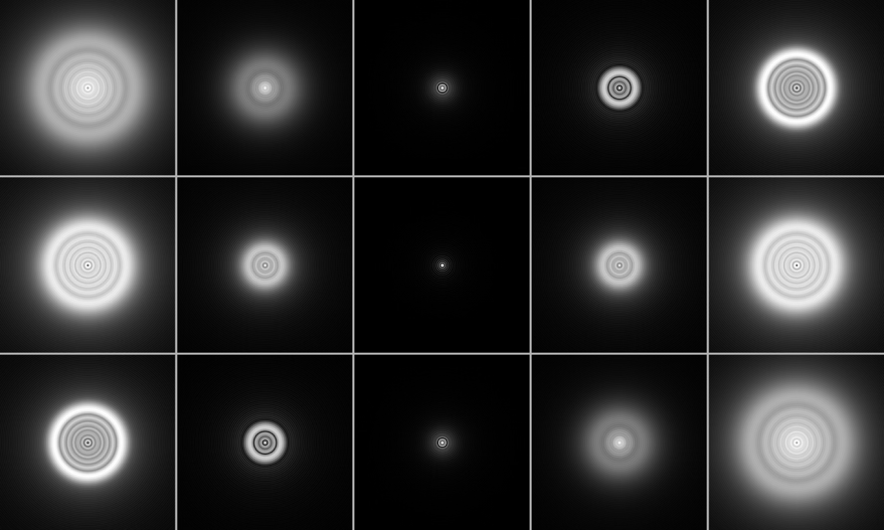
Top: diagram showing the effect of spherical aberration in an spherical mirror. Bottom: a set of images showing different levels of spherical aberration (left to right) at different focal positions (top to bottom).

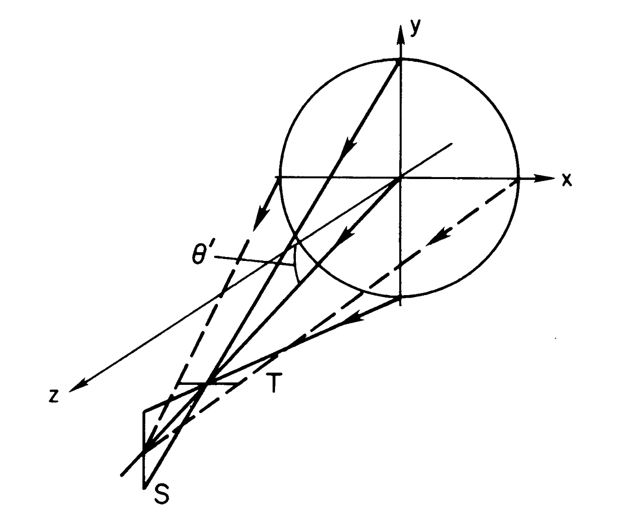
Coma

Coma is caused by different levels of magnification over the entrance pupil. The result is that off-axis point sources display a small tail or “comet-like” (coma) shape.

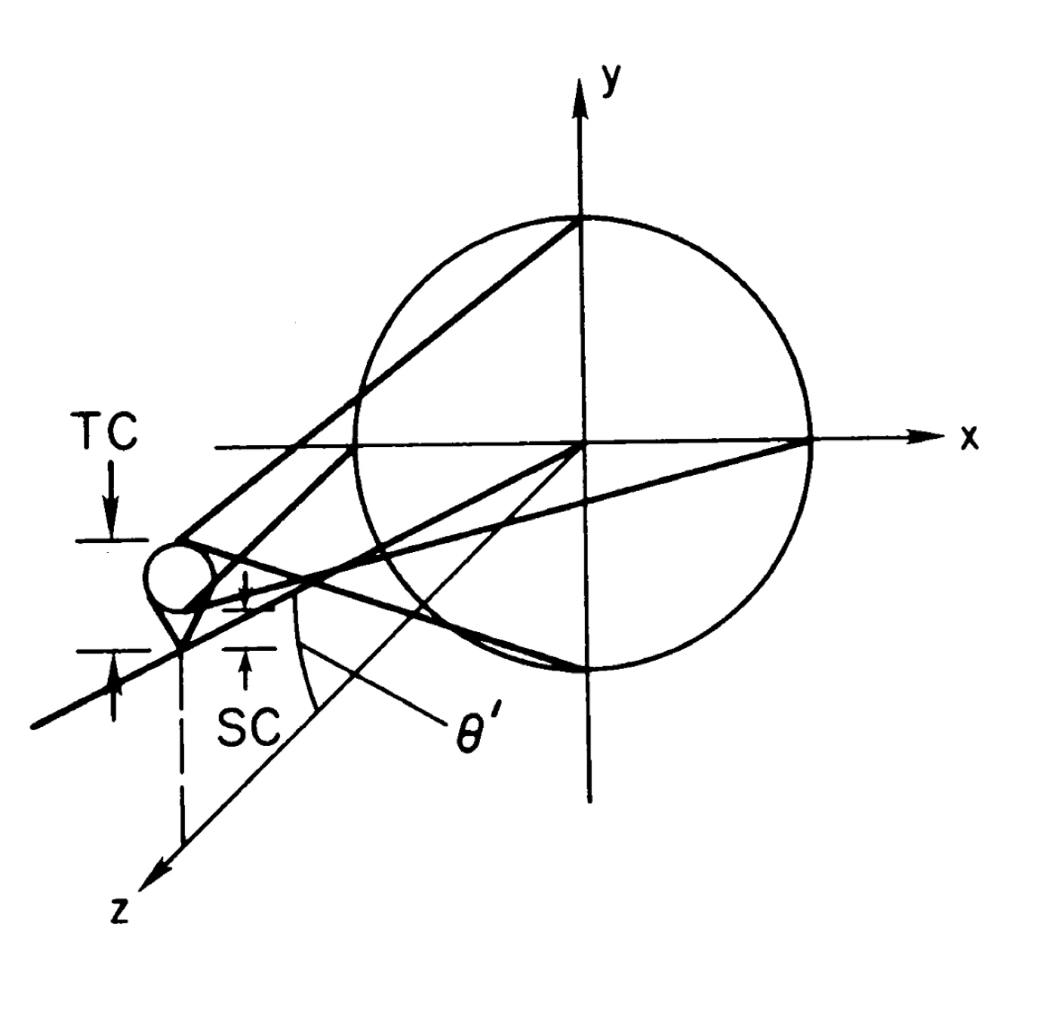
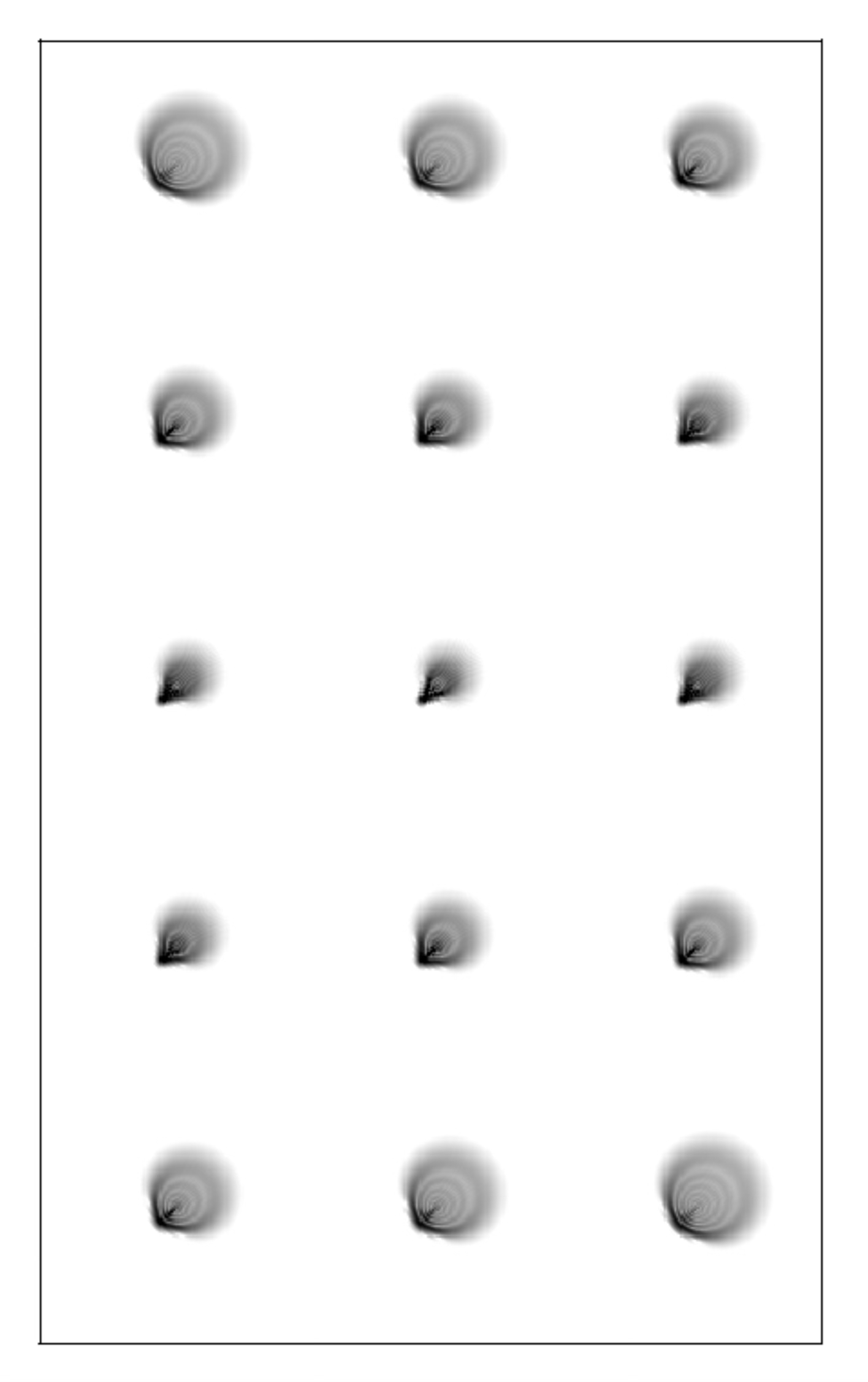
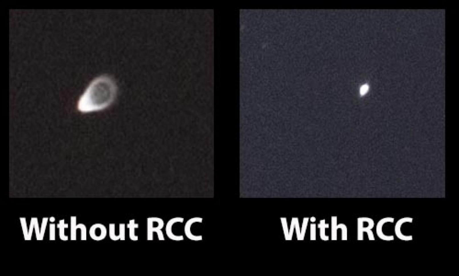
Top: diagram showing the effect of coma in a lens. Middle: a set of images showing the effect of comma in a point source image at different focal plane positions. Bottom: an example of coma being corrected using a corrector lens.

Astigmatism

Astigmatism is caused by the fact that the lens or mirror has different focal lengths for different orientations of the optical element. This means that a point source will be focused into an ellipse instead of a point. The effect is similar to coma, but the direction of the elongation of the ellipse depends on the orientation of the lens.

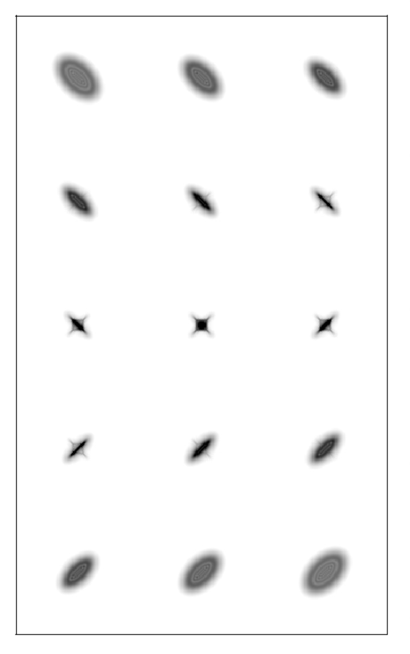
Top: diagram showing the effect of astigmatism in a lens. Bottom: a set of images showing the effect of astigmatism in a point source image at different focal plane positions. Note that while the direction of the coma does not change as we pass through focus, the astigmatism ellipse changes its orientation.

Diffraction

Although not technically an aberration, we will briefly discuss the effect of diffraction here. Diffraction is the bending of light, without changes to its energy, when the light passes through and aperture or obstacle. In optical systems the edges of mirrors or lenses can act as sources of diffraction. So far we have assumed that the wavelength of the light is much smaller than the aperture of the mirror, but in practice diffraction establishes the maximum resolution of the optical system, i.e., the smallest separation between two point sources that can be resolved.

It can be shown (see Schroeder, Astronomical Optics) that the diffraction limit of a circular aperture is given by

\[ R[\rm rad] = \dfrac{\lambda}{D} \]

where \(R\) is the resolution in radians, \(\lambda\) is the wavelength of the light, and \(D\) is the diameter of the aperture. For a one-metre telescope observing at \(5000\,\unicode{x212B}\), the resolution is about \(0.1\) arcseconds, which is less than what we be observed by ground-based telescopes due to atmospheric turbulence. In space, however, diffraction is often the limiting factor in the resolution of an optical telescope.

As we move to longer wavelengths the effect of diffraction becomes more important. The same telescope observing in the J band (1.25 \(\mu \rm m\)) has a resolution of about 0.25 arcseconds, while in the radio band (1 cm) the resolution is about 0.5 degrees. This means that radio telescopes need to be much larger than optical telescopes to achieve the same resolution.

Seeing

Another not-quite-an-aberration effect that affects ground-based telescopes is the seeing. Astronomical seeing is the perturbation of the light by the turbulence of air cells in the atmosphere and it’s usually the main factor limiting the resolution of ground-based telescopes. Seeing changes in relatively short timescales as the turbulence in the atmosphere changes. To first order, seeing has the effect of blurring the image of a point source into a Gaussian-like shape (sometimes a Lorentzian profile is more accurate). Because of this we often measure the seeing as the Full-Width at Half Maximum (FWHM) of the point spread function (PSF) of a star.

Astronomical observatories are located at high altitudes and in dry locations to reduce the effect of seeing. The best ground-based observatories often reach seeings of 0.2-0.3 arcseconds but often the seeing is worse than that and a seeing of 1 arcsec or more is common for many professional telescopes.

Seeing is a function of the altitude of the object on the sky, with the lowest seeing occurring when the object is at the zenith (and the light of the object has to pass through the least amount of atmosphere). The seeing can be related to the airmass, which is normally defined as the secant of the zenith angle of the object, \(X=\sec z=\sec (90-h)=\csc h\). With that definition, we can often approximate the seeing \(s\sim s_0 X^{3/5}\), where \(s_0\) is the seeing at the zenith.

Adaptive optics

The effect of seeing can sometimes be reduced by using adaptive optics. This technique uses a set of small mirrors that can be deformed to “undo” the effect of the seeing in the light wavefront. The mirrors are controlled by a computer that continuously monitors the image of a star and adjusts the shape of the mirrors to compensate for the distortion caused by the atmosphere. A wavefront sensor, usually located near the exit pupil, measured distortions in the wavefront and sends the information to a computer. This process is repeated many times per second.

An example of a distorted image. By knowing the distortion (the wavefront in the case of adaptive optics) we can deconvolve the original image. Credit: Wikipedia

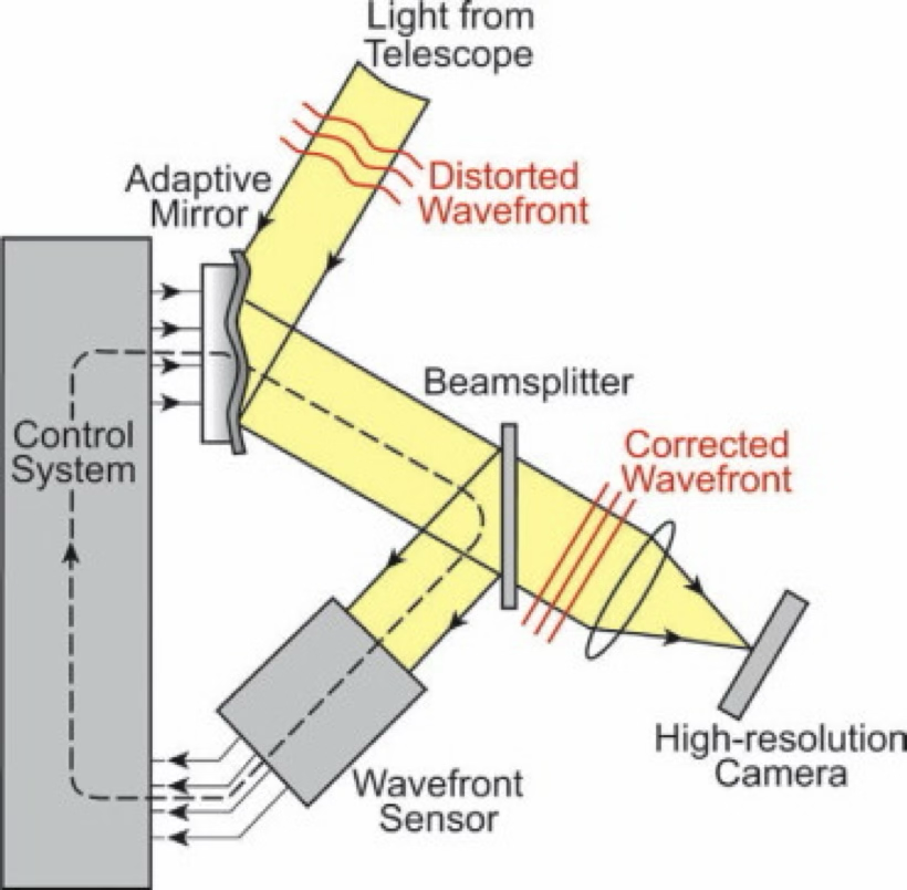
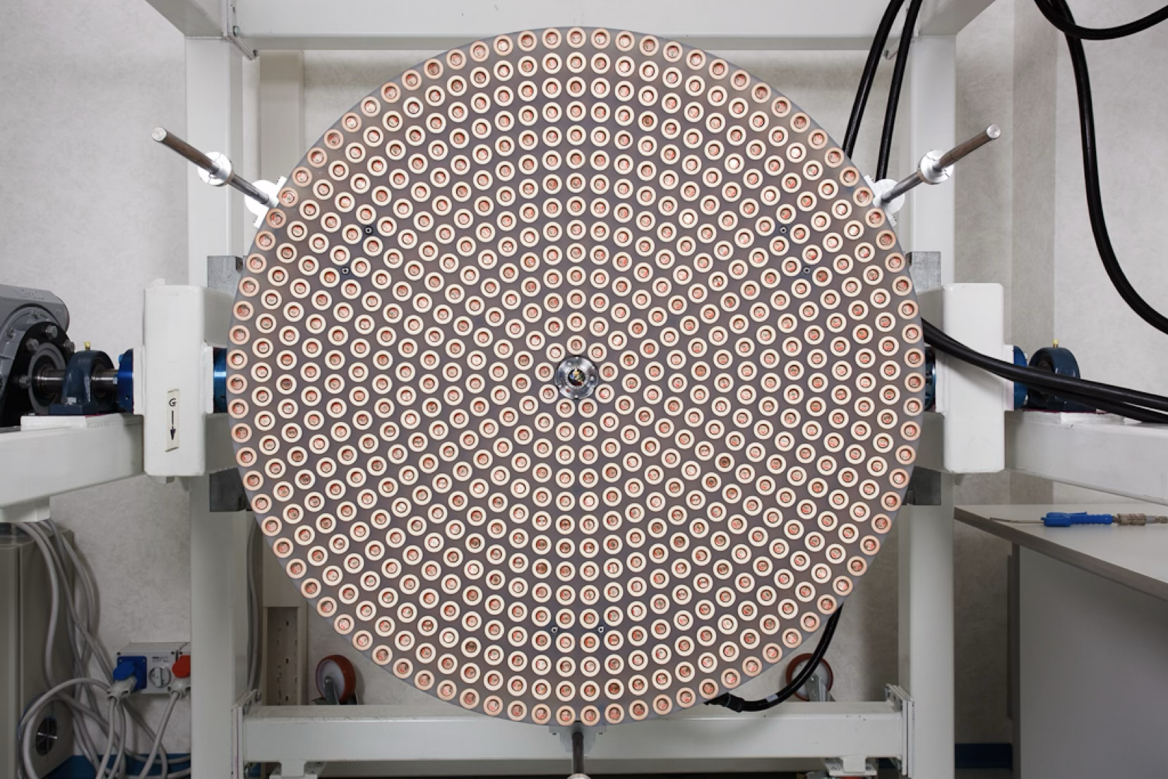
A diagram of an adaptive optics system (top) and a deformable mirror used to correct the wavefront (bottom).

Further reading

• Birney, D. S., Gonzalez, R. A., and Oesper, D. (2006). Observational Astronomy (2nd ed.)

• Smart, W. M. (1977). Textbook on Spherical Astronomy (6th ed.)

• Ryden, B., and Peterson, B. M. (2010). Foundations of Astronomy (3rd ed.)

• Schroeder, D., (2000) Astronomical Optics (2nd ed.)

• International Celestial Reference System